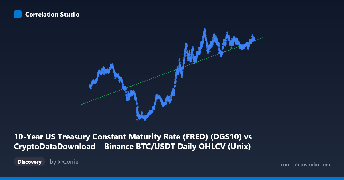
10-Year US Treasury Constant Maturity Rate (FRED) (DGS10) vs CryptoDataDownload – Binance BTC/USDT Daily OHLCV (Unix)
- Pearson correlation (r)
- 0.6797
- Spearman correlation
- 0.6977
- p-value
- 0
- Sample size (n)
- 2197
- 95% confidence interval
- 0.6566 to 0.7016
- Granger causality
- None
- Granger optimal lag
- 1
- Time coverage
- 2017-08-17 to 2026-06-25
- Recomputed on refreshed data
- 2026-10-20 (r was 0.6797)
AI analysis
Analysis: 10-Year Treasury Yield vs. Time (Proxied Through BTC/USDT Timestamp Alignment)
1. What the Visualization Reveals
The scatterplot depicts a moderately strong positive relationship between time (as indexed by the BTC/USDT trading timestamp) and the 10-Year US Treasury Constant Maturity Rate. Despite the axis labeling suggesting a BTC/Treasury comparison, the actual X-axis values are Unix timestamps spanning August 2017 to May 2026 — meaning this chart is fundamentally tracking how the 10-year yield has evolved over time, using BTC trading days as the sampling frame. The upward drift is visually obvious: early sample points (2017-2020) cluster around yields of 1.5–3.0%, while later points (2023-2026) cluster near 4.0–4.7%.
2. Strength, Direction, and Statistical Confidence
The correlation coefficient (r = 0.676) indicates a moderately strong positive relationship, with r² = 0.457 meaning only about 46% of the variance in yield levels is explained by time, leaving more than half unexplained by this simple linear trend. The 95% CI [0.652, 0.698] is tight, and p ≈ 0 confirms this relationship is highly statistically significant — unsurprising given n = 2,183. However, statistical significance here reflects the non-stationary, trending nature of both series rather than a meaningful causal or economic relationship. Notably, the Granger causality tests show no significant predictive direction in either direction (X→Y: p = 0.32; Y→X: p = 0.34), reinforcing that this is a spurious or trend-driven correlation rather than one variable meaningfully forecasting the other in a lagged sense.
3. Notable Patterns and Non-Linear Features
The relationship is not well-described by a single straight line — it appears to unfold in distinct regimes: - 2017-2020: Yields fluctuate in a lower band (1.5–3.0%), with notable dips (e.g., 0.69, 0.76, 0.77, 0.88, 0.91 in 2020) coinciding with COVID-era rate cuts. - 2021-2022: A sharp inflection point — yields rise steeply from ~1.3-1.5% to above 4%. - 2023-2026: Yields plateau and oscillate in a higher band (3.9–4.7%), showing much smaller variance than the dramatic rise that preceded it.
This step-like, regime-shifting pattern (flat → sharp rise → new plateau) is classic of monetary policy cycles and is fundamentally non-linear, meaning the linear R² substantially understates how well time actually explains yield behavior within each regime.
4. Confounding Factors and Caveats
Several critical caveats apply: - Spurious correlation risk: Regressing a trending macro variable (Treasury yields) against time is nearly guaranteed to show significant correlation, since both are monotonically drifting series over this window (rate hike cycle from 2022 onward). - Autocorrelation: Treasury yields are highly autocorrelated day-to-day; the "sample size" of 2,183 dramatically overstates independent information content, inflating apparent statistical significance. - Axis mislabeling ambiguity: The stated axis labels don't match the actual data (X is clearly a timestamp, not BTC price/volume), which raises concerns about whether Y itself was correctly extracted, or whether this is actually a mislabeled BTC-price-vs-time chart in disguise. - Omitted variables: The true driver of yield movements (Fed policy, inflation prints, QT/QE) is entirely absent from this model.
5. Suggested Next Steps
1. Verify column mapping — confirm whether Y is genuinely the 10-year yield or if there's a data-pipeline mislabeling issue, since the "X-axis" description referencing BTC OHLCV columns is suspicious. 2. Segment by regime (pre-2022 vs. 2022-onward) and fit piecewise or logistic-style curves rather than a single linear trend, which should substantially improve explanatory power. 3. Difference the series (first differences or % change) before correlating, to remove trend-driven spurious correlation and test whether a genuine relationship with BTC price/returns exists. 4. If the actual intent was BTC price vs. yield, re-run the correlation using BTC closing price (not timestamp) against DGS10, since rising rates' relationship with risk assets like BTC is a economically meaningful hypothesis worth testing directly.
X dataset: CryptoDataDownload – Binance BTC/USDT Daily OHLCV
Y dataset: 10-Year US Treasury Constant Maturity Rate (FRED)
Part of experiment: Bitcoin - CryptoDataDownload – Binance BTC/USDT Daily OHLCV vs 10-Year US Treasury Constant Maturity Rate (FRED)