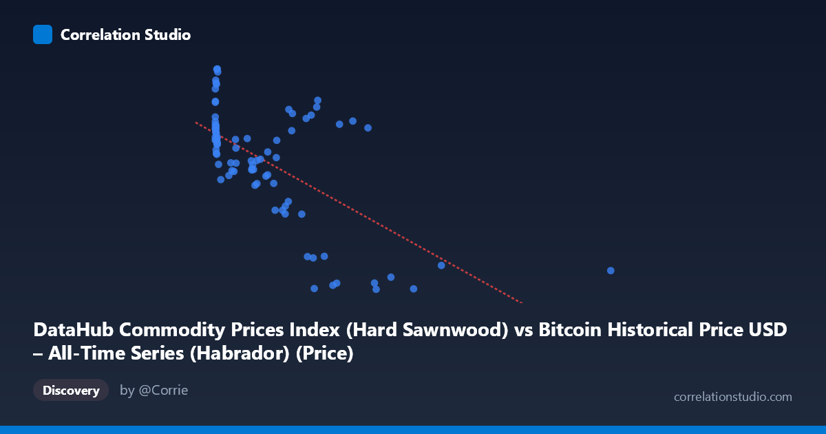
DataHub Commodity Prices Index (Hard Sawnwood) vs Bitcoin Historical Price USD – All-Time Series (Habrador) (Price)
- Pearson correlation (r)
- -0.6377
- Spearman correlation
- -0.5409
- p-value
- 0
- Sample size (n)
- 83
- 95% confidence interval
- -0.7502 to -0.4893
- Granger causality
- None
- Granger optimal lag
- 10
- Time coverage
- 2010-08-01 to 2017-06-01
- Recomputed on refreshed data
- 2026-10-24 (r was -0.6377)
AI analysis
Analysis: Hard Sawnwood Price Index vs. Bitcoin Historical Price (USD)
1. Overall Relationship
The scatterplot shows a moderate negative relationship between the two variables: as the "Hard Sawnwood" commodity index value (X) increases, the paired Bitcoin price value (Y) tends to decrease. The data is heavily right-skewed on the X-axis — the vast majority of points cluster below X=700, with a long tail of sparse points extending out to X=2452. This clustering pattern strongly influences the visual impression of the trend line.
2. Strength, Direction, and Statistical Confidence
The correlation coefficient (r = -0.638) indicates a moderate negative linear association, with r² = 0.407 meaning only about 41% of the variance in Y is explained by X — the majority (59%) is driven by other factors entirely. The 95% CI [-0.750, -0.489] is reasonably tight and excludes zero, and the p-value (8.99E-11) is highly significant, so we can be confident a real (non-zero) negative association exists in this sample — but the CI's width still reflects meaningful uncertainty about the precise strength of that relationship. Critically, the Granger causality tests show no significant predictive direction in either direction (X→Y: p=0.20; Y→X: p=0.22). This means that despite the contemporaneous correlation, neither series reliably helps forecast the other over time — the relationship is likely coincidental, structural, or driven by a shared external factor rather than genuine lead-lag causality.
3. Patterns, Clusters, and Outliers
The data shows two distinguishable regimes: a dense cluster of points with X < 700 spanning nearly the full Y range (672–974), and a sparse tail of high-X outliers (X 750, up to 2452) that consistently sit at lower Y values (roughly 670–905). This tail — including points like (2452.18, 697.44), (1402.08, 704.52), and (1230.02, 672.48) — is likely doing much of the work in producing the negative slope; without these few high-leverage points, the bulk cluster shows much weaker or noisier structure. Within the main cluster itself, there's no clean linear trend — Y values swing from ~672 to ~973 while X stays under 700, suggesting substantial scatter/noise independent of X in that region.
4. Confounding Factors and Caveats
This pairing is unusual and likely spurious: the X-axis label ("Hard Sawnwood" from a Bitcoin dataset) and Y-axis label ("Bitcoin Price" from a commodity index dataset) appear mismatched or mislabeled, suggesting a data-processing/column-swap error upstream. More fundamentally, both series may simply share a common time trend (2010–2017) — Bitcoin price grew explosively over this period while commodity indices had their own multi-year cycles, so any two time series with strong trends can show artificial correlation without genuine economic linkage. The small paired sample (n=83) versus full population (N=449) also means substantial data reduction/aliasing, and outliers in the high-X tail have outsized leverage on the correlation and regression slope.
5. Suggested Next Steps
Given the label confusion, the first priority should be verifying which variable actually belongs on which axis and confirming timestamps are correctly aligned between datasets. Next, the analysis should be rerun on detrended or differenced series (e.g., month-over-month % change) rather than raw levels, since trending series can produce misleading correlation/Granger results. Given the lack of Granger causality, this relationship should not be used for predictive/trading purposes; instead, treat it as coincidental co-movement and investigate whether a third factor (e.g., overall macroeconomic conditions, USD strength, or general risk sentiment 2010–2017) better explains both series' trajectories.
X dataset: Bitcoin Historical Price USD – All-Time Series (Habrador)
Y dataset: DataHub Commodity Prices Index
Part of experiment: Bitcoin - Bitcoin Historical Price USD – All-Time Series (Habrador) vs DataHub Commodity Prices Index