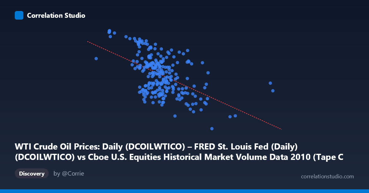
WTI Crude Oil Prices: Daily (DCOILWTICO) – FRED St. Louis Fed (Daily) (DCOILWTICO) vs Cboe U.S. Equities Historical Market Volume Data 2010 (Tape C Trade Count)
- Pearson correlation (r)
- -0.5219
- Spearman correlation
- -0.4645
- p-value
- 0
- Sample size (n)
- 252
- 95% confidence interval
- -0.6064 to -0.4258
- Granger causality
- None
- Granger optimal lag
- 1
AI analysis
Analysis: WTI Crude Oil Prices vs. Cboe Tape C Trade Count (2010)
Relationship Overview The scatterplot reveals a moderate negative relationship between WTI crude oil prices and Cboe Tape C trade counts during 2010. As oil prices rise, equity trade counts on Tape C tend to decline, and vice versa. The linear regression equation (y = -1.807×10⁻⁵x + 90.60) confirms this inverse slope, suggesting that for every roughly 55,000-unit increase in the oil price index (X), the trade count (Y) decreases by approximately one unit. Visually, the data points form a downward-sloping cloud with considerable scatter, indicating a real but imperfect relationship between these two variables across the trading year.
Correlation Strength and Statistical Significance The Pearson correlation of r = -0.522 reflects a moderate negative association. However, the R² of 0.272 is the more practical anchor here — it tells us that only about 27% of the variance in Tape C trade counts is explained by variation in WTI oil prices, meaning roughly 73% of the variation remains unexplained by this single predictor. With N = 3,302 and n = 252 paired observations, the result is statistically robust: the p-value is effectively 0, and the 95% confidence interval for r of [-0.606, -0.426] is comfortably negative throughout, ruling out a chance finding. That said, statistical significance here is partly a function of the large sample size rather than effect magnitude alone. Importantly, the Granger causality tests show no significant predictive directionality: neither oil prices predicting trade counts (F = 0.72, p = 0.397) nor trade counts predicting oil prices (F = 3.79, p = 0.053) clears the conventional α = 0.05 threshold. The Y→X result is borderline suggestive but falls just short, meaning we cannot claim a temporal lead-lag relationship between these two series at lag-1 with confidence.
Patterns, Clusters, and Outliers Several notable features emerge in the sampled data. There is a visible cluster of high trade counts (Y ≈ 85–91) concentrated at lower X values (roughly 300,000–500,000 range), suggesting that periods of lower oil prices coincided with heightened equity trading activity — potentially reflecting risk-on behavior or macro uncertainty driving volume. Conversely, high oil price observations (X 800,000–900,000) cluster at lower trade counts (Y ≈ 64–75). A standout outlier is the point at (1,379,287, 75.10) — the maximum X value — which sits far to the right of the main distribution yet its Y value is not extreme, potentially exerting leverage on the regression line. Similarly, (963,255, 64.78) represents the minimum Y value at a high X, reinforcing the negative trend. The spread of Y values at mid-range X values (500,000–700,000) is wide, suggesting high residual variance in the central portion of the distribution.
Confounding Factors and Caveats This correlation should be interpreted with considerable caution. Both series are likely driven by shared macroeconomic forces in 2010 — notably the post-financial crisis recovery, European sovereign debt concerns, and shifting risk appetite — rather than a direct causal mechanism between oil prices and equity trade volume. The axes appear to be switched relative to their dataset labels (WTI prices are on the X-axis but described as the Y dataset's source, and vice versa), which warrants careful verification before drawing operational conclusions. Additionally, equity trade counts are influenced by a vast array of factors (algorithmic trading activity, volatility regimes, earnings seasons, regulatory changes) that have nothing to do with oil. The single-year time window (2010) limits generalizability, and the non-linear scatter visible in the chart suggests that a linear model may be oversimplifying the true relationship structure.
Actionable Insights and Further Investigation Given the moderate correlation and absent Granger causality, practitioners should avoid using oil prices alone as a predictive signal for equity trade volume. However, the association is strong enough to warrant inclusion of oil prices as one feature in a multivariate model alongside volatility indices (e.g., VIX), macroeconomic indicators, and market regime variables. Researchers should investigate whether the relationship is regime-dependent — for instance, does the correlation strengthen during oil price shock periods? A rolling correlation analysis across multiple years would reveal whether the -0.52 correlation observed in 2010 is stable or an artifact of that particular macro environment. Testing non-linear models (e.g., piecewise regression or quantile regression) could better capture the apparent heteroscedasticity in the mid-range X values, and extending Granger causality tests to longer lags (beyond lag-1) may uncover delayed predictive relationships not captured in the current analysis.
X dataset: Cboe U.S. Equities Historical Market Volume Data 2010
Y dataset: WTI Crude Oil Prices: Daily (DCOILWTICO) – FRED St. Louis Fed (Daily)
Part of experiment: Daily - Cboe U.S. Equities Historical Market Volume Data 2010 vs WTI Crude Oil Prices: Daily (DCOILWTICO) – FRED St. Louis Fed (Daily)