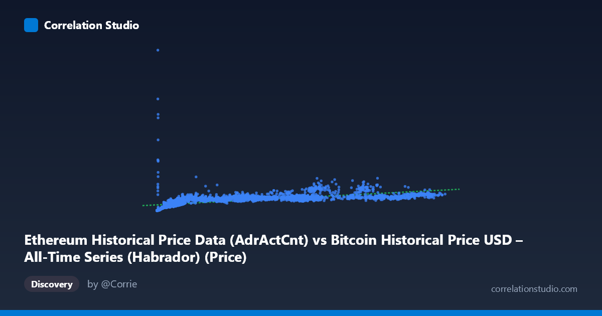
Ethereum Historical Price Data (AdrActCnt) vs Bitcoin Historical Price USD – All-Time Series (Habrador) (Price)
- Pearson correlation (r)
- 0.5775
- Spearman correlation
- 0.8901
- p-value
- 0
- Sample size (n)
- 3926
- 95% confidence interval
- 0.5563 to 0.598
- Granger causality
- None
- Granger optimal lag
- 10
AI analysis
Scatterplot Analysis: Ethereum AdrActCnt vs. Bitcoin Price USD
1. Overall Relationship
The visualization shows a positive but moderate association between the two variables, with values clustering heavily in the lower-left quadrant (X < 20,000; Y < 600,000) and thinning out into a sparse, more scattered upper range. The relationship appears non-linear: Y rises steeply as X moves from near-zero to roughly 5,000–10,000, then the rate of increase flattens considerably, producing a curve reminiscent of a logarithmic or power-law shape rather than a straight line. This is consistent with the note that Spearman ρ exceeds Pearson r — the rank-order relationship is stronger than the linear one, meaning a monotonic but curved fit would likely capture the pattern better than the linear equation (y = 5.32x + 258,442) currently does.
2. Strength, Direction, and Statistical Confidence
The Pearson correlation (r = 0.578) indicates a moderate positive relationship, with r² = 0.334 meaning only about 33% of the variance in Y is explained by X — leaving two-thirds of Y's variability attributable to other factors or non-linear dynamics not captured by this simple linear model. The 95% CI [0.556, 0.598] is tight, and the p-value of ~0 confirms the correlation is highly statistically significant and not a product of chance, given the large sample (n = 3,926). However, statistical significance here reflects sample size more than practical predictive strength — r² of 0.33 is modest. Critically, the Granger causality tests show no significant predictive direction in either direction (X→Y: p = 0.59; Y→X: p = 0.89), meaning neither variable's past values reliably forecast the other's future values at the tested lag structure. This suggests the correlation is likely driven by a shared underlying trend (e.g., both series generally rising over the 2015–2026 window) rather than one variable temporally leading the other.
3. Notable Patterns and Outliers
The data shows a dense cluster of points with X between roughly 200–20,000 and Y between 20,000–600,000, forming the core relationship. A secondary, sparser cluster exists at higher X values (60,000–125,000) where Y plateaus or even shows mild scatter without proportional increase — e.g., points near (72,688, 523,376) and (118,410, 744,255) don't scale linearly with the largest X values compared to smaller-X points like (75,892, 1,282,510), which is a clear outlier with disproportionately high Y. This flattening at high X, combined with an isolated high-Y spike at moderate X, suggests saturation effects or a distinct regime change — possibly corresponding to a specific market cycle (e.g., a Bitcoin bull run) where price surged independent of the X-axis metric's growth.
4. Confounding Factors and Caveats
The metadata reveals a significant labeling concern: the X-axis is described as Ethereum's Active Address Count while the dataset name says "Bitcoin Historical Price," and the Y-axis is labeled Bitcoin Price but sourced from an Ethereum dataset — this cross-labeling is confusing and should be verified before drawing asset-specific conclusions. Additionally, both series span 2015–2026 and likely share common macro drivers (crypto market cycles, adoption trends, speculative bubbles) that would inflate correlation without implying direct causation. Time-series data of this nature is also prone to autocorrelation and non-stationarity (trending series), which can artificially inflate Pearson r; the Granger test result reinforces that this is likely a spurious or trend-driven correlation rather than a causal linkage.
5. Recommendations for Further Investigation
Given the non-linear signal (Spearman Pearson), refitting with a log-log or power-law model would likely improve explanatory power substantially — I'd suggest testing y = a·ln(x) + b or a log-log linear regression first. Additionally, since both series appear non-stationary and Granger tests were insignificant, analysts should difference the data (e.g., day-over-day % changes) and re-run correlation/causality tests to check if the relationship holds after removing shared trend components. Finally, clarifying the true source/label of each axis (Bitcoin vs. Ethereum metrics) is essential before publishing conclusions, and segmenting the analysis by market cycle (bull/bear periods) may reveal that the relationship strength varies significantly by regime rather than being constant across the full time range.
X dataset: Bitcoin Historical Price USD – All-Time Series (Habrador)
Y dataset: Ethereum Historical Price Data
Part of experiment: Bitcoin - Bitcoin Historical Price USD – All-Time Series (Habrador) vs Ethereum Historical Price Data