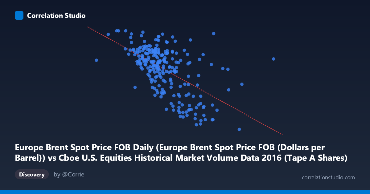
Europe Brent Spot Price FOB Daily (Europe Brent Spot Price FOB (Dollars per Barrel)) vs Cboe U.S. Equities Historical Market Volume Data 2016 (Tape A Shares)
- Pearson correlation (r)
- -0.5768
- Spearman correlation
- -0.5678
- p-value
- 0
- Sample size (n)
- 251
- 95% confidence interval
- -0.654 to -0.4879
- Granger causality
- None
- Granger optimal lag
- 1
AI analysis
Analysis: Europe Brent Spot Price vs. Cboe U.S. Equities Tape A Share Volume (2016)
Relationship Overview The scatterplot reveals a moderate negative relationship between Europe Brent crude oil spot prices (X-axis) and Cboe U.S. equities Tape A share volume (Y-axis) across 251 trading days in 2016. As oil prices increase, equity trading volume tends to decrease, and vice versa. The linear regression equation (y = -6.60×10⁻⁸x + 61.68) quantifies this inverse trend, though the scatter around the regression line is substantial, indicating that oil price alone is far from a complete explanation of trading volume behavior.
Correlation Strength and Statistical Interpretation The Pearson correlation of r = -0.5768 indicates a moderate negative association. However, the r² of 0.3328 means that only about 33.3% of the variance in Tape A share volume is explained by Brent crude prices — leaving roughly two-thirds of volume variation attributable to other factors. The 95% confidence interval of [-0.654, -0.488] is meaningfully narrow and entirely negative, reinforcing that the inverse relationship is genuine and not a statistical artifact. The p-value of effectively zero confirms strong statistical significance given the population size of 3,622. Critically, however, the Granger causality tests find no significant predictive directionality in either direction (X→Y: F=0.184, p=0.668; Y→X: F=0.494, p=0.483), meaning that past oil prices do not meaningfully predict future trading volume, nor does past trading volume predict future oil prices at the one-period lag tested. This distinguishes a contemporaneous correlation from a temporally actionable predictive signal.
Notable Patterns, Clusters, and Outliers The data exhibits a visibly heterogeneous distribution. A dense central cluster appears around oil prices of $220M–$290M (in the X-axis units representing daily notional volume proxies) and Tape A volumes of roughly 42–50 billion shares, suggesting a "normal" operating regime for most of 2016. Several notable outliers stand out: the point near (458M, 26) represents an extreme combination of high oil price and very low trading volume, while points near (176M–190M, 49–53) show high volume paired with low oil prices. The point cluster around (310M–365M, 27–33) suggests a regime where elevated oil prices coincided with markedly suppressed equity volume. There is also a hint of non-linearity, with volume appearing to plateau or compress in the mid-range of oil prices, which a purely linear model may underfit.
Confounding Factors and Caveats This correlation almost certainly reflects shared macroeconomic drivers rather than a direct causal mechanism between oil prices and equity trading volume. Both variables are plausibly influenced by risk-on/risk-off sentiment cycles, global growth expectations, Federal Reserve policy shifts, and broader financial market volatility (e.g., VIX spikes drive volume while suppressing oil in risk-off environments). The year 2016 was particularly event-rich — oil price recovery from multi-year lows, the U.S. presidential election, and Brexit uncertainty — all of which could independently drive both variables. Additionally, the axis labeling appears inverted in the dataset metadata (X is labeled from the Cboe dataset and Y from the Brent dataset), which warrants verification before drawing directional conclusions. The Granger causality null result further cautions against any mechanistic interpretation.
Actionable Insights and Further Investigation Given that one-third of volume variance is associated with oil prices but no temporal predictive relationship exists, practitioners should avoid using daily oil price changes as a leading indicator for equity volume forecasting. More productive next steps would include: (1) incorporating additional covariates such as VIX, macroeconomic data releases, or sector-specific flows to build a multivariate volume model; (2) testing Granger causality at longer lags (2–5 periods) to detect slower-moving relationships; (3) segmenting the data by market regime (low vs. high volatility periods) to assess whether the correlation strengthens conditionally; and (4) investigating whether the relationship is driven by specific sectors (e.g., energy equities) or is broad-based across Tape A listings. The outlier observations at extreme oil price levels warrant individual examination to determine whether they correspond to identifiable market events.
X dataset: Cboe U.S. Equities Historical Market Volume Data 2016
Y dataset: Europe Brent Spot Price FOB Daily
Part of experiment: Daily - Cboe U.S. Equities Historical Market Volume Data 2016 vs Europe Brent Spot Price FOB Daily