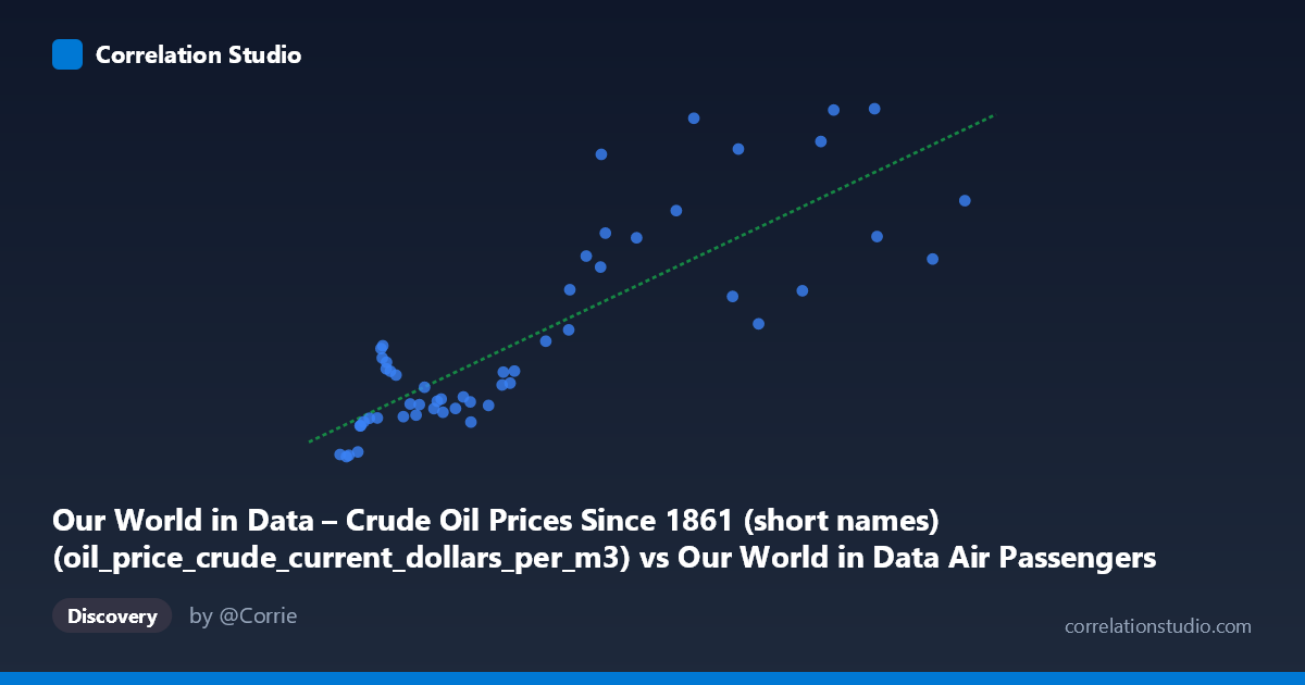
Our World in Data – Crude Oil Prices Since 1861 (short names) (oil_price_crude_current_dollars_per_m3) vs Our World in Data Air Passengers Carried (Air transport, passengers carried)
- Pearson correlation (r)
- 0.8358
- Spearman correlation
- 0.8321
- p-value
- 0
- Sample size (n)
- 54
- 95% confidence interval
- 0.7318 to 0.9017
- Granger causality
- None
- Granger optimal lag
- 10
AI analysis
Analysis: Crude Oil Prices vs. Air Passengers Carried (1970–2023)
1. Overall Relationship
The scatterplot reveals a clear positive association between crude oil prices (in current dollars per cubic meter) and global air passengers carried. As oil prices rise, air passenger numbers tend to increase rather than decrease — a counterintuitive finding at first glance. The linear regression equation (y = 4.69×10⁻⁶x + 31.93) confirms this upward trajectory, with both variables trending strongly upward across the 1970–2023 time window. This suggests that rather than reflecting a direct causal mechanism, both variables are primarily being driven by a shared underlying force: long-run global economic growth and rising prosperity.
2. Correlation Strength, Direction, and Causality
The Pearson correlation of r = 0.836 indicates a strong positive linear relationship, and the R² of 0.699 means approximately 70% of the variance in air passenger volumes is statistically explained by oil price variation in this paired sample — a substantial proportion. The 95% confidence interval for r of [0.732, 0.902] is relatively tight and lies entirely in positive territory, reinforcing that this association is robust and not a sampling artifact. The p-value of 3.78×10⁻¹⁵ is extraordinarily small, confirming the correlation is highly statistically significant for n = 54 paired observations drawn from a population of N = 164.
However, the Granger causality results critically undercut any temporal predictive interpretation. Neither direction reaches conventional significance: X→Y yields F = 2.07, p = 0.072, and Y→X yields F = 1.38, p = 0.252 — even at an optimal lag of 10 periods. This means oil prices do not reliably predict future passenger volumes, and passenger volumes do not predict future oil prices. The correlation, however strong statistically, does not encode a directional predictive signal useful for forecasting in either direction.
3. Notable Patterns, Clusters, and Outliers
Several structural features are visible in the data:
- Lower-left cluster (oil prices ~8–35M USD/m³, passengers ~11–150): This likely represents the 1970s–1990s era, when both aviation was less accessible and oil, while volatile, remained at historically lower nominal levels. Points like (9,374,736, 11.32) and (8,087,298, 15.60) anchor this cluster. - Mid-range dispersion (oil prices ~40–70M, passengers ~100–460): Considerable vertical scatter here — for similar oil price levels, passenger counts vary widely (e.g., ~113 vs. ~455 at roughly similar X values). This heteroscedasticity suggests the linear model is less precise in this range. - Upper-right outliers of note include (107,771,284, 699.78), (116,013,260, 702.38), and (79,529,812, 683.44) — extremely high passenger counts possibly reflecting post-2010 aviation expansion in Asia-Pacific, particularly China and India. Conversely, (127,744,044, 403.87) and (134,258,317, 519.80) show high oil prices but relatively moderate passenger numbers, possibly reflecting pandemic-era or price-shock disruptions. - The spread widens substantially at higher X values, indicating heteroscedasticity — variance in Y grows with X — which violates a key assumption of ordinary least squares regression and suggests a log-linear or power-law model might fit better.
4. Confounding Factors and Interpretive Caveats
This correlation is almost certainly spurious in a causal sense, driven by several confounds:
- Shared time trend: Both variables rise secularly over 1970–2023 due to global economic expansion, population growth, and inflation. Without detrending, any two upward-trending time series will appear correlated. - Nominal oil prices: The X-axis uses current (nominal) dollar prices, meaning inflation alone mechanically inflates X over time, artificially strengthening the correlation with any other nominally growing variable. - Aggregation effects: Air passengers are likely aggregated across countries or globally, masking regional heterogeneity (e.g., Middle East aviation booming precisely because of oil wealth). - Oil price shocks vs. trends: Major disruptions (1973 OPEC embargo, 1979 shock, 2008 financial crisis, 2020 COVID collapse) should theoretically produce negative short-run relationships between oil prices and travel demand — yet these are obscured by the long-run trend. - Reverse logic: High oil revenues enable sovereign wealth and consumer spending in oil-exporting regions, potentially increasing air travel demand during high-price periods, adding a non-obvious positive feedback.
5. Actionable Insights and Further Investigation
Given the ambiguous causal structure, several follow-up analyses are warranted:
- Detrend both series (e.g., first-differencing or HP filter) before computing correlation to isolate cyclical co-movement from shared secular trends — this will likely substantially reduce r. - Use real (inflation-adjusted) oil prices, which are available in the source dataset, to remove the mechanical nominal inflation effect. - Re-run Granger causality at shorter lags (1–3 periods) where economic theory would predict oil price shocks to affect travel decisions, and consider structural break tests around 2008 and 2020. - Segment analysis: Separate the dataset by decade or by region (OECD vs. emerging markets) — the relationship may be strongly positive in oil-exporting economies and weakly negative or neutral in oil-importing ones. - Incorporate GDP as a covariate: A partial correlation controlling for GDP per capita would likely reveal whether oil prices retain any explanatory power once economic growth is accounted for. - Explore log-log transformation: Given visible heteroscedasticity and the likely power-law nature of both variables' growth, a log-linear model may yield better-calibrated residuals and a more interpretable elasticity coefficient.
Bottom line: The strong statistical correlation (r = 0.836, R² = 0.699) between crude oil prices and air passengers is real but almost certainly reflects shared long-run economic trends rather than a direct causal mechanism. The absence of Granger causality in either direction confirms this. Analysts should resist policy or commercial conclusions drawn from this correlation without first controlling for inflation, GDP growth, and temporal autocorrelation.
X dataset: Our World in Data Air Passengers Carried
Y dataset: Our World in Data – Crude Oil Prices Since 1861 (short names)
Part of experiment: Yearly - Our World in Data Air Passengers Carried vs Our World in Data – Crude Oil Prices Since 1861 (short names)