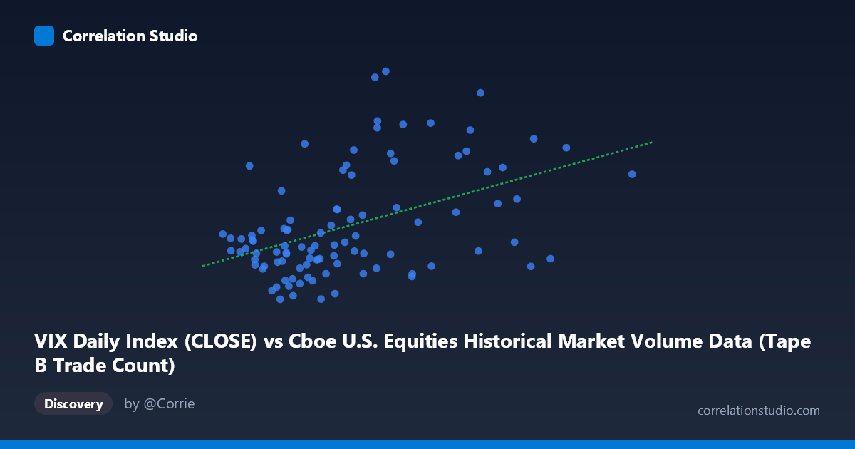
VIX Daily Index (CLOSE) vs Cboe U.S. Equities Historical Market Volume Data (Tape B Trade Count)

Pearson correlation (r): 0.4515
Spearman correlation: 0.3974
p-value: 0.000003
Sample size (n): 99
95% confidence interval: 0.2789 to 0.5958
Granger causality: None
Granger optimal lag: 1

AI analysis

Scatterplot Analysis: VIX vs. Tape B Trade Count

Relationship Overview

The scatterplot reveals a positive relationship between the VIX Daily Index (Close) and Cboe U.S. Equities Historical Market Volume (Tape B Trade Count), suggesting that as market volatility — as measured by the VIX — rises, trading activity on Tape B venues tends to increase. The linear regression equation (y = 7.105E-06x + 12.644) reflects this upward slope, consistent with the intuitive notion that heightened fear or uncertainty in equity markets drives greater trading volume. However, the relationship is clearly noisy, with substantial scatter around the regression line, indicating that VIX alone is far from a complete predictor of Tape B trade counts.

Correlation Strength and Statistical Significance

The Pearson correlation of r = 0.4515 indicates a moderate positive association, but the explanatory power is modest: R² = 0.2038, meaning VIX explains only about 20.4% of the variance in Tape B trade counts, leaving nearly 80% attributable to other factors. The 95% confidence interval of [0.2789, 0.5958] is meaningfully above zero and reasonably tight given the sample size (n = 99), lending credibility to the direction of the effect. The p-value of 2.727E-06 is highly statistically significant, strongly rejecting the null hypothesis of no linear relationship. However, the Granger causality tests yield no significant result in either direction (X→Y: F = 0.0006, p = 0.98; Y→X: F = 0.0004, p = 0.98), meaning that past values of VIX do not meaningfully predict future Tape B trade counts at a one-period lag, and vice versa. This is a critical caveat: statistical correlation does not imply temporal predictive causation here, and the relationship may be largely contemporaneous or driven by shared underlying forces.

Notable Patterns, Clusters, and Outliers

Several features stand out visually. The bulk of observations cluster in the X range of roughly 650,000–1,100,000 with Y values between approximately 14.5 and 22, forming a dense core. Above X ≈ 1,100,000, points become more sparse but tend toward higher Y values, consistent with the positive trend. There are notable high-leverage outliers: the point near (1,115,472, 31.05) and (1,085,027, 30.61) sit well above the regression line, as does (1,091,495, 26.95), suggesting occasional spikes in Tape B activity that the VIX level alone doesn't fully explain. Conversely, points like (1,578,717, 17.44) and (1,523,838, 16.88) show very high X values but surprisingly low Y values, pulling against the trend and hinting at non-linearity or regime-specific behavior at extreme volume levels. The relationship may plateau or even invert at very high market volumes.

Confounding Factors and Caveats

Several important caveats apply. First, the axes appear to be swapped in labeling — the dataset descriptions suggest VIX values should be in a range of roughly 10–80, yet the X-axis spans ~657,000 to ~1,808,758, which is more consistent with trade counts, not VIX levels. This warrants careful verification of the data pipeline before drawing conclusions. Second, even if the labels are correct, macroeconomic events, earnings seasons, index rebalancing, and market structure changes (e.g., exchange fee changes, fragmentation) could independently drive both VIX and trade counts, creating spurious correlation. Third, the time coverage is narrow (January–May 2026, just under five months), limiting generalizability and potentially capturing a single market regime. Finally, with N = 1,980 population points but only n = 99 sampled, sampling variability could influence the observed correlation.

Actionable Insights and Further Investigation

Given the moderate but statistically robust correlation and the absence of Granger causality, practitioners should not use VIX as a leading indicator for short-term Tape B trade count forecasting in isolation. Instead, further investigation should: (1) verify and correct the axis/dataset labeling to ensure variables are mapped correctly; (2) explore non-linear models (e.g., polynomial regression, LOESS smoothing) given the visible scatter and potential plateau effects at extremes; (3) introduce control variables such as market cap, Tape A/C volumes, and macroeconomic surprises to build a more complete predictive model; (4) extend the time series across multiple years to test whether this relationship is stable across different volatility regimes (e.g., 2020 COVID spike, 2022 rate-hike cycle); and (5) investigate the high-outlier cluster around X ≈ 1,085,000–1,115,000 with Y 30 to determine whether specific market events explain the anomalous trade activity.

X dataset: Cboe U.S. Equities Historical Market Volume Data

Y dataset: VIX Daily Index

Part of experiment: Daily - Cboe U.S. Equities Historical Market Volume Data vs VIX Daily Index