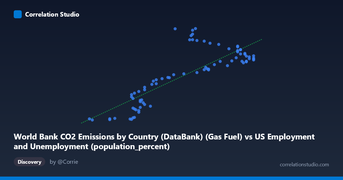
World Bank CO2 Emissions by Country (DataBank) (Gas Fuel) vs US Employment and Unemployment (population_percent)
- Pearson correlation (r)
- 0.8171
- Spearman correlation
- 0.7774
- p-value
- 0
- Sample size (n)
- 80
- 95% confidence interval
- 0.7281 to 0.879
- Granger causality
- None
- Granger optimal lag
- 10
- Time coverage
- 1941-01-01 to 2020-01-01
AI analysis
Scatterplot Analysis: Gas Fuel CO2 Emissions vs. US Employment Population Percent
1. Overall Relationship Pattern
The scatterplot reveals a positive, moderately strong relationship between gas fuel CO2 emissions and US employment as a percentage of population, spanning annual observations from 1941 to 2020. As gas fuel CO2 emissions increase along the x-axis (ranging from roughly 55.8 to 67.1 units), employment population percentages trend upward substantially — from lows near 654 to highs approaching 17,000. However, the relationship is visually heteroscedastic: variance in Y expands dramatically at higher X values, and a pronounced fan-shaped spread is evident in the mid-to-upper X range (~62–64 units), suggesting the linear model captures central tendency but masks considerable complexity at higher emission levels.
2. Correlation Strength, Direction, and Causality
The Pearson correlation of r = 0.817 indicates a strong positive association, and the linear regression equation (y = 1205.57x − 66,503.5) confirms a steep positive slope. However, r² = 0.668 means that approximately 66.8% of the variance in Y is explained by X, leaving roughly one-third of variability unaccounted for — a meaningful residual that the scatterplot makes visually apparent. The 95% confidence interval for r [0.728, 0.879] is relatively tight and well above zero, and the p-value ≈ 0 confirms this correlation is highly statistically significant with virtually no probability of arising by chance in a sample of n = 80. That said, the Granger causality results are unambiguous in their null finding: neither X→Y (F = 0.859, p = 0.576) nor Y→X (F = 1.590, p = 0.138) achieves significance at any conventional threshold, even at the optimal lag of 10 periods. This means that neither variable temporally predicts the other — the correlation, however strong statistically, carries no demonstrated predictive directionality over time.
3. Notable Patterns, Clusters, and Outliers
Several structural features stand out. A lower-left cluster of points (X ≈ 55.8–60.0, Y < 5,000) forms a relatively tight grouping, likely representing mid-20th century observations when both emissions and employment metrics were lower. In the middle X range (62–64), Y values scatter extremely widely — from approximately 8,000 to nearly 17,000 — which is the primary driver of unexplained variance and signals that some third force is operating. Points at (62.7, 14,984), (62.9, 16,694), (62.8, 15,736), (62.9, 15,999), and (63.1, 16,992) are notable high-Y outliers clustered around similar X values, suggesting specific historical episodes (possibly post-WWII employment booms or specific economic expansions) where employment surged independently of emission levels. Several low-Y outliers at moderate X (e.g., ~58.6, 830; ~58.7, 768; ~56.0, 654) likely represent early wartime or Depression-adjacent years. The overall shape hints at a possible non-linear or segmented relationship rather than a purely linear one.
4. Confounding Factors and Interpretive Caveats
The most critical caveat is that this analysis appears to combine data from two conceptually unrelated datasets — US employment statistics and global CO2 emissions by country — joined on time (year) rather than any causal mechanism. The strong r likely reflects shared temporal trends: both gas fuel CO2 emissions and employment population percentages grew substantially across the 20th century due to industrialization, population growth, and economic expansion, making them spuriously correlated through time as a common confounder. The axis labels also warrant scrutiny — "Gas Fuel CO2 Emissions" appearing in a US Employment dataset column, and vice versa, suggests potential data joining artifacts or mislabeling. Heteroscedasticity violates linear regression assumptions and inflates uncertainty at higher X values. Additionally, the 80-year time span (1941–2020) encompasses World War II, multiple recessions, the 2008 financial crisis, and the COVID-19 pandemic, all of which would independently perturb both variables in ways unrelated to any structural relationship between them.
5. Actionable Insights and Further Investigation
Given the absence of Granger causality, this correlation should not be used for forecasting or policy inference without substantially deeper analysis. Recommended next steps include: (1) detrending both series (e.g., first-differencing or HP filtering) to remove shared secular trends before re-estimating correlation, which will likely reduce r dramatically; (2) testing for structural breaks at known economic events (WWII end, 1973 oil shock, 2008 crisis, 2020 pandemic); (3) exploring non-linear models (polynomial or piecewise regression) given the evident heteroscedasticity and the wide Y-scatter at mid-range X; (4) examining whether the relationship holds within sub-periods rather than pooling 80 years; and (5) clarifying the data provenance and join logic to confirm these variables are correctly matched and that the dataset column attributions are accurate before drawing any substantive conclusions.
X dataset: US Employment and Unemployment
Y dataset: World Bank CO2 Emissions by Country (DataBank)
Part of experiment: Yearly - US Employment and Unemployment vs World Bank CO2 Emissions by Country (DataBank)