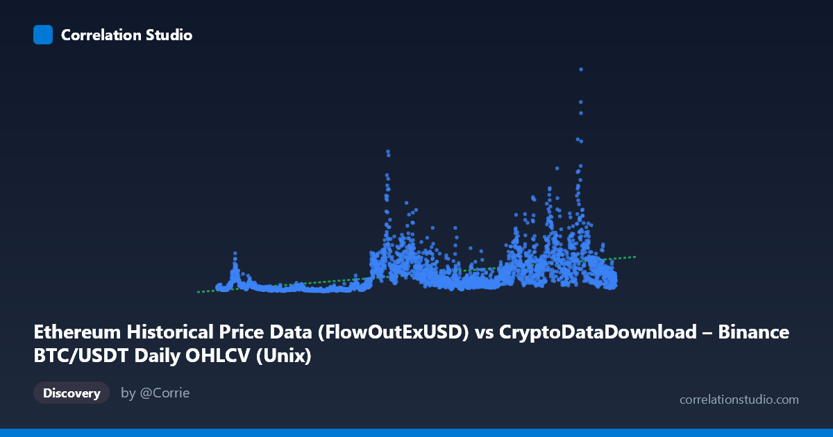
Ethereum Historical Price Data (FlowOutExUSD) vs CryptoDataDownload – Binance BTC/USDT Daily OHLCV (Unix)
- Pearson correlation (r)
- 0.4792
- Spearman correlation
- 0.6385
- p-value
- 0
- Sample size (n)
- 3191
- 95% confidence interval
- 0.452 to 0.5055
- Granger causality
- None
- Granger optimal lag
- 10
- Time coverage
- 2017-08-17 to 2026-05-20
AI analysis
Analysis: Ethereum Flow-Out (X) vs. Binance BTC/USDT Metric (Y)
1. What the Visualization Reveals
The scatterplot shows a moderate positive relationship between the X variable (timestamped, spanning 2017–2026) and Y, with substantial scatter around the regression line. Given that X is actually a time-indexed series (Unix timestamps) rather than a true independent variable, this plot is functionally showing how Y has trended over roughly nine years. The wide dispersion — Y ranges from ~$13.9M to ~$7.36B (a 500x spread) while X progresses linearly — suggests the relationship is driven more by distinct market regimes (bull/bear cycles) than a smooth, continuous trend.
2. Strength, Direction, and Uncertainty
The correlation coefficient (r = 0.479) indicates a moderate positive relationship, but r² = 0.230 means only 23% of the variance in Y is explained by time/X — the remaining 77% is driven by other factors (volatility, market cycles, external shocks). The 95% CI [0.452, 0.505] is tight, and p ≈ 0 confirms this correlation is highly statistically reliable, not a product of chance — but statistical significance here reflects the large sample size (n=3,191) more than practical predictive strength.
Critically, the Granger causality tests show no significant predictive direction (X→Y: p=0.22; Y→X: p=0.23). This means neither series meaningfully helps forecast the other's future values based on past values — despite the contemporaneous correlation, there's no evidence of a lead-lag relationship. This is an important distinction: correlation without Granger causality suggests both series may be responding to a common external driver (e.g., overall crypto market sentiment, macro liquidity cycles) rather than one causing the other.
3. Notable Patterns and Non-linearity
The data shows clear clustering by market era: early samples (2017–2020) cluster tightly at low Y values (~$60M–$230M), while 2021 onward shows dramatic expansion with values reaching into the billions, interspersed with pullbacks (e.g., 2022–2023 samples dropping back to $220M–$500M range). This is consistent with BTC/ETH bull-bear cycles rather than a linear trend. The note that Spearman ρ exceeds Pearson r strongly suggests a non-linear (likely logarithmic or power-law) relationship — typical of financial/volume data with exponential growth phases. A log-transform of Y (common for volume/price-driven metrics) would likely improve model fit substantially.
4. Confounding Factors and Caveats
Several caveats apply: - Autocorrelation: Both series are time-series with strong internal momentum (trends, cycles), which inflates apparent correlation and violates independence assumptions underlying the p-value. - Common driver: Bitcoin and Ethereum markets are both influenced by shared macro factors (interest rates, regulatory news, overall crypto sentiment) — the correlation may be spurious in a causal sense, reflecting shared exposure to these drivers rather than a direct relationship between the named variables. - Non-stationarity: Cryptocurrency volume/flow data typically exhibits regime shifts and heteroskedasticity, undermining linear regression assumptions (constant variance, linearity). - Data labeling ambiguity: The axis descriptions are unusually structured (X described as an Ethereum flow-out metric, but sourced from BTC/USDT OHLCV; Y labeled as Binance BTC/USDT Unix-time data, but described as Ethereum metrics) — this suggests potential data mapping or column-labeling errors that should be verified before drawing conclusions.
5. Recommendations for Further Investigation
1. Re-verify column/axis mapping — the source/label mismatch (BTC data described as Ethereum metrics) should be resolved before further analysis. 2. Apply log transformation to Y (and possibly X-detrending) to test whether a log-linear model substantially improves R², given the Spearman/Pearson divergence. 3. Decompose by market regime (e.g., bull vs. bear years) to check if correlation strength varies by period — pooled correlation may mask regime-specific relationships. 4. Test differenced/returns data rather than levels, since Granger causality and correlation on raw trending series can produce misleading results; re-run Granger tests on stationary (differenced) series. 5. Investigate shared external covariates (e.g., total crypto market cap, USD liquidity indices) as potential common causes driving both series simultaneously.
X dataset: CryptoDataDownload – Binance BTC/USDT Daily OHLCV
Y dataset: Ethereum Historical Price Data
Part of experiment: Bitcoin - CryptoDataDownload – Binance BTC/USDT Daily OHLCV vs Ethereum Historical Price Data