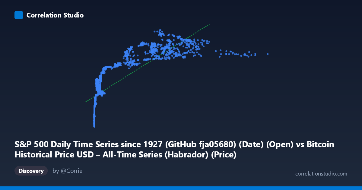
S&P 500 Daily Time Series since 1927 (GitHub fja05680) (Date) (Open) vs Bitcoin Historical Price USD – All-Time Series (Habrador) (Price)
- Pearson correlation (r)
- 0.7845
- Spearman correlation
- 0.9422
- p-value
- 0
- Sample size (n)
- 2376
- 95% confidence interval
- 0.7686 to 0.7995
- Granger causality
- X → Y
- Granger optimal lag
- 1
AI analysis
Analysis: Bitcoin Price vs. S&P 500 Time Series Relationship
Important caveat on labeling: The column headers appear swapped/mismatched — the "X-axis" is described as an S&P 500 column but its values (0.05 to 18,960) and scale clearly represent Bitcoin's price history, while the "Y-axis" (1,046 to 3,226) with far lower volatility looks more like an equity index. The analysis below treats X as Bitcoin price and Y as the S&P 500-like series, but this metadata inconsistency should be resolved before drawing firm conclusions.
1. What the Visualization Reveals
The scatterplot shows a clear positive, but strongly non-linear relationship. At low X-values (under ~1,000), Y rises steeply and then curves — data points cluster tightly between Y=1,200 and Y=2,200 while X moves from near 0 to about 1,000. Beyond that, as X stretches out to nearly 19,000, Y increases only modestly further, plateauing between roughly 2,600 and 3,200. This is a classic logarithmic/saturating growth pattern rather than a straight line.
2. Strength, Direction, and Statistical Confidence
The Pearson correlation (r = 0.7845, R² = 0.6155) indicates a strong positive linear association explaining ~61.6% of variance in Y — meaningful, but leaving nearly 40% unexplained by a straight-line model. The tight 95% CI [0.7686, 0.7995] and p≈0 confirm this correlation is highly statistically reliable given n=2,376, not a chance artifact. However, the note that Spearman ρ exceeds Pearson r is a strong signal: the true relationship is monotonic but curved (likely logarithmic), meaning a log-transformed X would likely explain substantially more variance than the current linear R².
The Granger causality result adds a temporal dimension: X→Y is significant (F=6.43, p=0.0113) while Y→X is not (p=0.0879). This suggests X's past values have modest predictive power for future Y values beyond Y's own history, but not vice versa — consistent with unidirectional lead-lag behavior at 1-period lag. This is suggestive of temporal precedence, not proof of causation.
3. Notable Patterns and Outliers
The data show three regimes: (1) a dense cluster at X<1,000 where Y ranges widely (1,200–2,400) — high sensitivity at low X; (2) a mid-range (1,000–10,000) with fewer points but continued Y growth; (3) a sparse high-X tail (X10,000) where Y compresses into a narrow 2,600–3,200 band, indicating diminishing marginal effect — a textbook logarithmic ceiling. No sharp discontinuities or reversals are evident, but the compression at high X could also reflect fewer observations (survivorship in later years) rather than a true asymptote.
4. Confounding Factors and Caveats
Both series span 2010–2019, a period when nearly all major asset classes trended upward due to macro factors like near-zero interest rates, quantitative easing, and general bull markets — a classic spurious-correlation risk from shared time trends rather than direct interaction. Neither series is stationary (both show strong secular growth), which can inflate correlation and distort Granger causality tests; results should be re-run on differenced/returns data rather than price levels. Additionally, the metadata mismatch between axis labels raises data-integrity concerns.
5. Suggestions for Further Investigation
1. Verify/correct column-dataset labeling before any further modeling. 2. Re-fit using log(X) given the Spearman/Pearson discrepancy — likely to raise explained variance substantially. 3. Test cointegration and run Granger causality on returns/log-differences, not raw levels, to control for trend-driven spurious correlation. 4. Segment analysis by year or regime (e.g., pre/post 2017 Bitcoin bubble) to check whether the relationship is stable or driven by specific episodes.
X dataset: Bitcoin Historical Price USD – All-Time Series (Habrador)
Y dataset: S&P 500 Daily Time Series since 1927 (GitHub fja05680) (Date)
Part of experiment: Bitcoin - Bitcoin Historical Price USD – All-Time Series (Habrador) vs S&P 500 Daily Time Series since 1927 (GitHub fja05680) (Date)