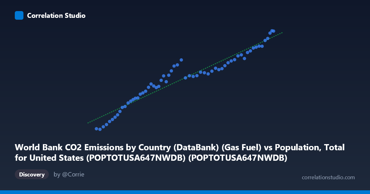
World Bank CO2 Emissions by Country (DataBank) (Gas Fuel) vs Population, Total for United States (POPTOTUSA647NWDB) (POPTOTUSA647NWDB)
- Pearson correlation (r)
- 0.9615
- Spearman correlation
- 0.9781
- p-value
- 0
- Sample size (n)
- 61
- 95% confidence interval
- 0.9364 to 0.9768
- Granger causality
- None
- Granger optimal lag
- 10
AI analysis
Scatterplot Analysis: U.S. Population vs. Gas Fuel CO₂ Emissions (1960–2020)
1. Overall Relationship
The scatterplot reveals a strong, positive, and largely linear relationship between total U.S. population and gas fuel CO₂ emissions over the 1960–2020 period. As population grows from roughly 181 million to 332 million, gas fuel emissions rise correspondingly from approximately 4,170 to 16,992 units, tracing what appears to be a smooth, continuous upward arc across six decades. The data points cluster tightly around the fitted regression line (y = 7.098×10⁻⁵x − 7,306.5), indicating that the growth in both variables has been remarkably synchronized over time — a hallmark of two variables that are both primarily driven by the passage of time and underlying economic expansion.
2. Correlation Strength, Direction, and Causality
The Pearson correlation of r = 0.9615 is exceptionally strong and positive, and the coefficient of determination R² = 0.9245 means that approximately 92.5% of the variance in gas fuel CO₂ emissions is statistically explained by variation in U.S. population size within this sample. The 95% confidence interval for r spans [0.9364, 0.9768], which is notably narrow and lies entirely in high-correlation territory, indicating very low uncertainty about the strength of this association. The p-value of effectively zero confirms that this correlation is astronomically unlikely to arise by chance under the null hypothesis of no relationship. However, the Granger causality tests complicate the causal interpretation significantly: neither X→Y (F = 0.533, p = 0.853) nor Y→X (F = 0.642, p = 0.767) achieves statistical significance even at an optimal lag of 10 periods. This means that neither variable meaningfully predicts future changes in the other beyond what is already captured by their shared temporal trend — a critical caveat against concluding that population growth drives emissions, or vice versa.
3. Notable Patterns, Clusters, and Outliers
The data points form a remarkably clean, nearly monotonic progression with no dramatic clustering by era or obvious breakpoints. There is mild visual suggestion of a slight non-linear (concave) curvature in the lower-population range (roughly 181–210 million, corresponding to 1960s data), where emissions may rise somewhat more steeply per unit of population, potentially reflecting the energy-intensive industrialization of that period. In the upper range (300+ million, post-2000), a few points show minor scatter above the trend line, possibly corresponding to years of economic expansion or unusually cold winters driving natural gas demand. No dramatic outliers are evident, though the point near (252 million, 13,202) sits modestly above the regression line, as does the cluster around 244–250 million, suggesting a period of slightly elevated emissions relative to population size. The high-population tail (320 million) appears remarkably consistent with the linear fit.
4. Confounding Factors and Interpretive Caveats
The most important caveat here is spurious correlation driven by shared time trend: both U.S. population and gas fuel CO₂ emissions have grown monotonically over the study period, and nearly any two such trending series will produce a high r value. The Granger causality results confirm this suspicion — the predictive content disappears once the temporal structure is properly accounted for. Additional confounders include GDP growth, which co-trends with both population and energy consumption; energy price shocks (e.g., 1970s oil crises, which may have shifted consumption toward or away from gas); technological efficiency changes and the shale gas revolution of the 2000s–2010s, which dramatically altered natural gas availability and cost; and structural economic shifts from manufacturing toward services. The regression equation also implies a non-trivial negative intercept (−7,306), which is physically meaningless at low population values, flagging that the linear model is an approximation valid only within the observed range.
5. Actionable Insights and Further Investigation
Given the near-perfect collinearity driven by time, the most productive next steps would be to detrend both series (e.g., using first differences or per-capita normalization) before re-examining correlation and causality — this would isolate whether year-over-year changes in population size actually correspond to changes in gas emissions, independent of the shared growth trend. Analysts should also investigate gas emissions per capita as the more policy-relevant metric, which would reveal whether emissions intensity has risen, fallen, or plateaued over the period. Incorporating GDP, energy prices, heating degree days, and industrial output as control variables in a multivariate model would help disentangle the population signal from broader economic drivers. Finally, extending the Granger causality test across a range of shorter lags (1–5 periods) rather than relying solely on the optimal lag of 10 would provide a more robust picture of any short-term temporal dynamics that the current test may be obscuring.
X dataset: Population, Total for United States (POPTOTUSA647NWDB)
Y dataset: World Bank CO2 Emissions by Country (DataBank)
Part of experiment: Yearly - Population, Total for United States (POPTOTUSA647NWDB) vs World Bank CO2 Emissions by Country (DataBank)