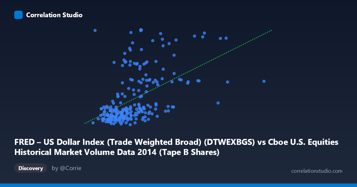
FRED – US Dollar Index (Trade Weighted Broad) (DTWEXBGS) vs Cboe U.S. Equities Historical Market Volume Data 2014 (Tape B Shares)
- Pearson correlation (r)
- 0.5134
- Spearman correlation
- 0.5629
- p-value
- 0
- Sample size (n)
- 245
- 95% confidence interval
- 0.4148 to 0.6001
- Granger causality
- None
- Granger optimal lag
- 1
AI analysis
Scatterplot Analysis: US Dollar Index vs. Cboe Tape B Share Volume (2014)
Relationship Overview The scatterplot reveals a moderate positive relationship between the US Dollar Index (Trade Weighted Broad) on the x-axis and Cboe Tape B Shares on the y-axis across 245 trading days in 2014. The linear regression equation (y = 5.26×10⁻⁸x + 91.639) indicates that as the dollar index rises, Tape B share values tend to increase modestly. However, the scatter is considerable, and a striking visual feature is the presence of what appears to be two distinct clusters or behavioral regimes in the data — a dense concentration of points at lower Y values (roughly 93–96) and a secondary grouping at elevated Y values (97–102), suggesting the relationship is not uniformly linear across the full range.
Correlation Strength and Statistical Significance The Pearson correlation of r = 0.5134 indicates a moderate positive association, but the explained variance of r² = 0.2636 means that only about 26.4% of the variance in Tape B Shares is attributable to variation in the Dollar Index — leaving nearly three-quarters of the variation unexplained by this relationship alone. The 95% confidence interval of [0.4148, 0.6001] is reasonably tight and does not cross zero, lending credibility to the direction of the association. The p-value of effectively zero (given N = 3,686) confirms statistical significance, though this should be interpreted cautiously given the large population size, which inflates power substantially. Critically, Granger causality tests in both directions fail to reach significance (X→Y: F = 0.040, p = 0.842; Y→X: F = 0.235, p = 0.628), meaning neither variable reliably predicts the other temporally at a one-period lag. The correlation, while real, does not appear to reflect a directional, predictive causal mechanism at this timescale.
Notable Patterns, Clusters, and Outliers The data exhibits a clear bimodal vertical structure: the majority of observations cluster tightly between Y ≈ 93–96 across a wide range of X values, while a distinct upper cluster sits between Y ≈ 97–102, also spanning a broad X range. This pattern strongly suggests a categorical or regime-switching dynamic rather than a smooth continuous relationship. Several notable outliers are visible — particularly points with very high X values (e.g., ~161M and ~196M) that do not follow the dominant trend, and high-Y points at moderate X values (e.g., ~40M X with Y ≈ 102.30, and ~100M X with Y ≈ 101.99). These outliers exert disproportionate influence on the regression slope and correlation coefficient, potentially inflating r.
Confounding Factors and Caveats Several important caveats apply. First, the axis labels appear to be swapped in the dataset metadata — the X-axis is described as market volume data while its column name references FRED's Dollar Index, and vice versa; this warrants verification before drawing substantive conclusions. Second, both variables are time series measured daily throughout 2014, making them susceptible to serial autocorrelation, which can artificially inflate Pearson correlation estimates. Third, macroeconomic confounders — such as Federal Reserve policy shifts, earnings seasons, geopolitical events, and general risk-on/risk-off sentiment — could simultaneously drive both dollar strength and equity trading volumes, producing a spurious or mediated correlation. The bimodal Y distribution further suggests an omitted categorical variable (e.g., market structure changes, exchange-specific policy events, or seasonal effects) driving the regime separation independently of the dollar index.
Actionable Insights and Further Investigation Given the bimodal structure, the most productive next step would be to identify and label the two clusters — examining whether the upper Y regime corresponds to specific dates, market events, or exchange rule changes in 2014. Researchers should also apply time series-appropriate methods such as cointegration testing or dynamic conditional correlation models, rather than relying solely on static Pearson correlation. Extending the Granger causality test to multiple lags (beyond just lag 1) could reveal delayed predictive relationships. Additionally, partial correlation analysis controlling for market-wide volume, VIX, or Fed policy indicators would help isolate whether the dollar-volume relationship is genuine or entirely mediated by broader macro conditions. Finally, resolving the apparent axis/metadata labeling inconsistency is essential before any policy or trading conclusions are drawn from this analysis.
X dataset: Cboe U.S. Equities Historical Market Volume Data 2014
Y dataset: FRED – US Dollar Index (Trade Weighted Broad)
Part of experiment: Daily - Cboe U.S. Equities Historical Market Volume Data 2014 vs FRED – US Dollar Index (Trade Weighted Broad)