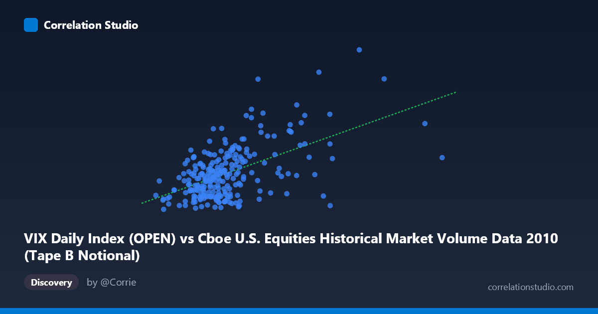
VIX Daily Index (OPEN) vs Cboe U.S. Equities Historical Market Volume Data 2010 (Tape B Notional)
- Pearson correlation (r)
- 0.5461
- Spearman correlation
- 0.4443
- p-value
- 0
- Sample size (n)
- 252
- 95% confidence interval
- 0.4532 to 0.6274
- Granger causality
- Y → X
- Granger optimal lag
- 1
AI analysis
Analysis: VIX Open vs. Tape B Notional Value (2010)
Relationship Overview The scatterplot reveals a positive relationship between the VIX Daily Index opening values and Tape B Notional trading volume, meaning that as market volatility (VIX) increases, the notional value of trades on Tape B exchanges tends to rise as well. This is broadly intuitive: heightened volatility typically drives increased trading activity as market participants react to uncertainty, hedge positions, or seek opportunistic entries. The linear regression equation (y = 1.42489E⁻⁰⁹x + 15.3751) confirms this upward slope, though the relatively modest coefficient suggests the relationship, while real, is far from deterministic.
Correlation Strength and Statistical Significance The correlation coefficient of r = 0.546 indicates a moderate positive association, but the more telling statistic is r² = 0.298 — meaning only approximately 29.8% of the variance in Tape B Notional is explained by VIX Open levels. The remaining ~70% of variation is attributable to other factors entirely. The 95% confidence interval of [0.453, 0.627] is reasonably narrow given the sample size of 252, and the p-value of effectively zero confirms this is not a chance finding. Critically, the Granger causality analysis points unidirectionally: Y Granger-causes X (F = 5.73, p = 0.017), meaning past VIX values appear to predict future Tape B notional volume, but not vice versa (F = 1.60, p = 0.208). This is a meaningful directional signal — volatility sentiment appears to lead trading volume activity, not the other way around, at least at a 1-period lag.
Notable Patterns, Clusters, and Outliers The data exhibits several visually distinct features. The bulk of observations cluster in the lower-left region — VIX values roughly between 15–25 and notional volumes in the 3–6 billion range — reflecting the relatively calm, recovering market conditions for much of 2010. However, there is a notable upper tail with a handful of extreme outliers: one point near (11.8B, 47.66) and another near (9.8B, 43.15) stand out dramatically, representing periods of significant simultaneous spikes in both volume and volatility. These likely correspond to specific market stress events (e.g., the May 2010 Flash Crash). There also appears to be heteroscedasticity — variance in Y increases substantially at higher X values — suggesting the linear model may underfit the high-volatility regime, and a log transformation or piecewise model might better capture the dynamics.
Confounding Factors and Caveats Several important caveats apply. First, Tape B specifically covers NYSE American (AMEX) and regional exchange securities, which may not uniformly reflect broad market behavior — structural factors unique to that tape could independently influence notional values. Second, the 2010 timeframe is not ordinary: it encompasses post-financial crisis recovery, the Flash Crash of May 6, and evolving high-frequency trading dynamics, all of which could artificially inflate the observed correlation. Third, the Granger causality result, while statistically suggestive, does not establish economic causation — omitted variables such as macroeconomic news releases, Fed announcements, or institutional rebalancing schedules could simultaneously drive both series. Finally, the large gap between N (3,302) and n (252) warrants attention; if this sample is not representative of the full population, inference may be limited.
Actionable Insights and Further Investigation The finding that VIX Granger-causes Tape B notional volume at a 1-day lag has practical implications for intraday and next-day liquidity planning — traders and market makers on Tape B exchanges could use VIX open levels as a leading indicator for expected volume and adjust inventory or quoting strategies accordingly. For further investigation, it would be valuable to: (1) test non-linear models (e.g., polynomial or log-log regression) given the apparent heteroscedasticity; (2) isolate the Flash Crash period and rerun the analysis to determine whether the correlation holds outside of that extreme event; (3) extend the Granger analysis to longer lags to see if predictive power persists beyond one period; and (4) compare across Tape A and Tape C to assess whether this VIX-volume relationship is exchange-structure-specific or a universal U.S. equity market phenomenon.
X dataset: Cboe U.S. Equities Historical Market Volume Data 2010
Y dataset: VIX Daily Index
Part of experiment: Daily - Cboe U.S. Equities Historical Market Volume Data 2010 vs VIX Daily Index