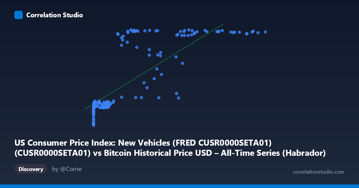
US Consumer Price Index: New Vehicles (FRED CUSR0000SETA01) (CUSR0000SETA01) vs Bitcoin Historical Price USD – All-Time Series (Habrador) (Price)
- Pearson correlation (r)
- 0.8226
- Spearman correlation
- 0.8595
- p-value
- 0
- Sample size (n)
- 193
- 95% confidence interval
- 0.7709 to 0.8635
- Granger causality
- None
- Granger optimal lag
- 1
- Time coverage
- 2010-08-01 to 2026-08-01
- Recomputed on refreshed data
- 2026-10-24 (r was 0.8133)
AI analysis
Analysis: Bitcoin Price vs. US New Vehicle CPI
1. What the Visualization Reveals
Despite the axis labels (which appear swapped in the metadata — the actual X variable is Bitcoin price and Y is new vehicle CPI, based on the data ranges), the scatterplot shows a clear non-linear, saturating relationship rather than a clean linear trend. At low X values (roughly 0–10,000), Y clusters tightly in a narrow band around 143–148. As X increases past ~20,000, Y jumps sharply upward into the 176–179 range, with a scattered transitional zone between ~30,000–60,000 where values swing widely (149 to 179). This pattern looks more like a step-function or logistic curve than a straight line — consistent with two variables that are each trending over time (CPI inflation and Bitcoin's long-term price appreciation) rather than one directly driving the other.
2. Strength, Direction, and Uncertainty
The Pearson r = 0.813 (r² = 0.662) indicates a strong positive association, with 66% of Y's variance statistically explained by X in a linear model. The 95% CI [0.759, 0.857] is reasonably tight given n=189, and p≈0 confirms the correlation is not due to chance. However, r² leaves 34% of variance unexplained, and the visual pattern suggests the true relationship is non-linear (the linear fit likely understates the strength at extremes and overstates it in the middle transition zone). Critically, the Granger causality tests show no significant predictive direction in either direction (X→Y: p=0.859; Y→X: p=0.309). This is a crucial caveat: strong correlation without Granger causality strongly suggests both series are independently trending upward over time (a classic spurious-correlation-via-common-trend scenario), rather than one variable causing or forecasting the other.
3. Notable Patterns and Outliers
Three distinct regimes are visible: (a) a dense low-X cluster (X < 10,000) with Y tightly bound between 142–148, representing most of the earlier/lower-value observations; (b) a sparse "transition" zone (X ≈ 30,000–60,000) with high variance in Y (149 to 179) — this is where the relationship is least stable and most poorly explained by a linear model; (c) a high-X cluster (X 60,000) where Y consistently sits at 177–179, suggesting Y has plateaued or is bounded by a ceiling (or measurement scale) independent of further increases in X. This ceiling effect is a strong signal of non-linearity that r² alone cannot capture.
4. Confounding Factors and Caveats
Both series are monotonically trending over a long time span (2010–2026), and CPI for new vehicles and Bitcoin price are both influenced by macroeconomic factors like inflation, monetary policy, and time itself — not by each other. This is a textbook case where time is the likely lurking confounder: both variables generally rose over the sample period for unrelated structural reasons (Bitcoin's adoption/speculative cycles vs. vehicle price inflation from supply chain and monetary policy). The lack of Granger causality reinforces that this is very likely a spurious or coincidental correlation driven by shared temporal trend rather than genuine economic linkage.
5. Actionable Insights
Analysts should avoid interpreting this r²=0.66 as evidence of a causal or tradeable relationship between Bitcoin price and vehicle CPI. Recommended next steps: (1) detrend or difference both series (e.g., using % change or log-returns rather than levels) and re-run the correlation to check if it persists — trending series often show spurious high correlation in levels that vanishes in differences; (2) test for cointegration rather than simple correlation, given both are non-stationary trending series; (3) segment the analysis by time period (pre-2020 vs. post-2020) to see if the relationship is stable or an artifact of concurrent bull markets; (4) if a genuine link is suspected (e.g., inflation driving both consumer prices and speculative asset demand), consider adding a common macro variable (CPI overall, M2 money supply, or interest rates) as a control in a multivariate model.
X dataset: Bitcoin Historical Price USD – All-Time Series (Habrador)
Y dataset: US Consumer Price Index: New Vehicles (FRED CUSR0000SETA01)
Part of experiment: Bitcoin - Bitcoin Historical Price USD – All-Time Series (Habrador) vs US Consumer Price Index: New Vehicles (FRED CUSR0000SETA01)