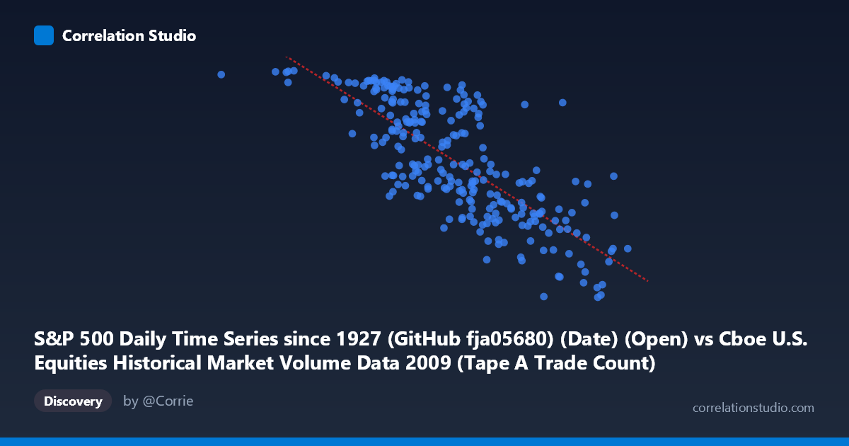
S&P 500 Daily Time Series since 1927 (GitHub fja05680) (Date) (Open) vs Cboe U.S. Equities Historical Market Volume Data 2009 (Tape A Trade Count)
- Pearson correlation (r)
- -0.7729
- Spearman correlation
- -0.7803
- p-value
- 0
- Sample size (n)
- 252
- 95% confidence interval
- -0.8183 to -0.7179
- Granger causality
- X → Y
- Granger optimal lag
- 10
AI analysis
S&P 500 Opening Price vs. Cboe Tape A Trade Count (2009)
Relationship Overview The scatterplot reveals a clear negative relationship between the S&P 500 daily opening price and Cboe Tape A trade count throughout 2009. As the S&P 500 index opened at higher price levels, the number of trades on Tape A (NYSE-listed securities) tended to decline. This pattern is economically intuitive given the context of 2009: the year began in the depths of the financial crisis, when equity prices were depressed and market participants — including panicked retail investors, institutional rebalancers, and high-frequency traders responding to volatility — were executing an exceptionally high volume of trades. As prices recovered through the year, the frenetic trading activity characteristic of crisis conditions subsided.
Correlation Strength and Statistical Significance The Pearson correlation of r = -0.7729 indicates a strong negative linear association, and the R² of 0.5974 means that roughly 59.7% of the variance in Tape A trade counts is explained by the S&P 500 opening price level — a substantial explanatory share for a single-variable model in financial data. The 95% confidence interval of [-0.8183, -0.7179] is relatively narrow and lies entirely in negative territory, confirming robustness of the directional finding. The p-value of effectively zero removes any doubt about statistical significance. Critically, the Granger causality analysis indicates a unidirectional temporal predictive relationship: S&P 500 opening prices Granger-cause Tape A trade counts at a 10-period lag (F = 1.9736, p = 0.0373), while the reverse direction fails to reach significance (F = 1.5309, p = 0.1296). This suggests that price level movements have predictive information about future trading activity, though causation in the strict economic sense warrants further scrutiny.
Notable Patterns, Clusters, and Outliers Several structural features stand out. There is a visible cluster of high trade-count observations at lower price levels (roughly X < 800,000–900,000 on the transformed axis, corresponding to early 2009 crisis lows), where trade counts frequently exceed 1,050–1,128. Conversely, as prices rise above ~2,000,000 on the X scale, trade counts compress into a narrower band around 700–900. A handful of outliers are apparent: the point near (362,081; 1,121) represents an extreme low-price, high-activity day — likely a crisis panic session — while points near (2,387,937; 679) and (2,549,192; 776) sit at the high-price, low-activity extreme. The relationship also shows mild heteroscedasticity: variance in trade counts is wider at lower price levels and narrows as prices rise, suggesting the linear model may slightly misfit the lower end of the distribution.
Confounding Factors and Caveats Several important caveats apply. First, both variables are strongly time-trending in 2009 — prices rose from March lows while trading activity gradually normalized — meaning the correlation may substantially reflect a shared temporal trend rather than a direct structural relationship between price level and trading volume. This is a classic spurious correlation driven by a common underlying driver (recovery from the financial crisis). Second, Tape A trade count specifically captures NYSE-listed securities, so fragmentation effects — trading migrating to dark pools or other venues — could distort the count independently of price movements. Third, the 10-period Granger lag is meaningful but modest in predictive F-statistic terms, suggesting the predictive signal, while statistically present, may not be large in practical magnitude. Finally, the linear regression slope (-0.000229 per unit of X) produces sensible fitted values but the heteroscedasticity noted above means prediction intervals will be unreliable at price extremes.
Actionable Insights and Further Investigation Practitioners and researchers should consider detrending both series (e.g., by removing the common time trend or using first-differences) to isolate whether a genuine structural relationship exists beyond the shared recovery trajectory. It would be valuable to extend the analysis across multiple years — particularly including non-crisis years — to test whether the negative correlation persists or is unique to 2009's extraordinary conditions. Incorporating implied volatility (VIX) as a control variable would help disentangle whether it is price level per se or the associated volatility regime driving trade counts. Given the Granger result, a rolling-window forecasting model using lagged S&P 500 prices to predict near-term Tape A activity could be tested for practical trading operations or market surveillance purposes. Finally, examining other tape categories (B and C) alongside total notional value would clarify whether this phenomenon is exchange-specific or market-wide.
X dataset: Cboe U.S. Equities Historical Market Volume Data 2009
Y dataset: S&P 500 Daily Time Series since 1927 (GitHub fja05680) (Date)
Part of experiment: Daily - Cboe U.S. Equities Historical Market Volume Data 2009 vs S&P 500 Daily Time Series since 1927 (GitHub fja05680) (Date)