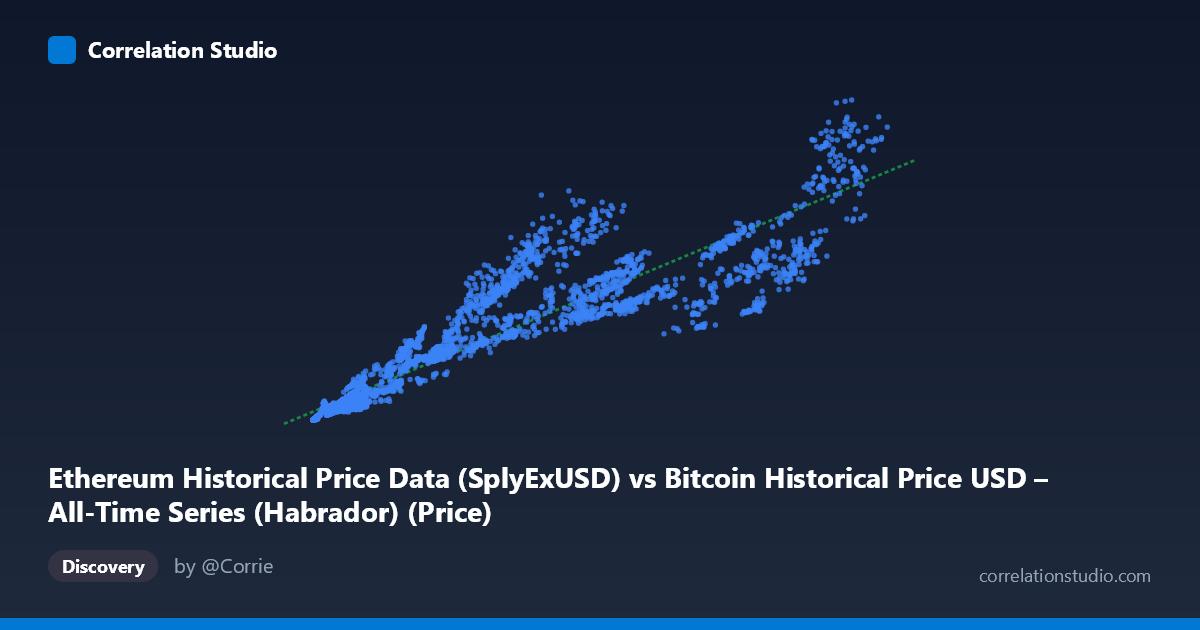
Ethereum Historical Price Data (SplyExUSD) vs Bitcoin Historical Price USD – All-Time Series (Habrador) (Price)
- Pearson correlation (r)
- 0.9249
- Spearman correlation
- 0.967
- p-value
- 0
- Sample size (n)
- 3917
- 95% confidence interval
- 0.9203 to 0.9293
- Granger causality
- None
- Granger optimal lag
- 10
AI analysis
Analysis: Ethereum Supply (SplyExUSD) vs. Bitcoin Historical Price
1. Overall Relationship
The scatterplot depicts a strong, positive, monotonic relationship between the X variable (labeled as Ethereum's SplyExUSD metric, though the value ranges suggest this is actually a price-like series) and Y (Bitcoin price in USD). As X increases from near-zero (~209) to its maximum (~124,720), Y climbs from a few million dollars up to nearly $96 billion. The data points trace a fairly consistent upward trajectory, though a closer look at the sample points reveals meaningful scatter around the fitted line, particularly at higher X values — suggesting the relationship may steepen (convex/super-linear) rather than remain purely linear across the full range.
2. Correlation Strength and Predictive Direction
With r = 0.9249 and r² = 0.8555, roughly 86% of the variance in Y is statistically explained by X — a strong linear association. The 95% confidence interval [0.9203, 0.9293] is tight, and the p-value of effectively 0 confirms this correlation is highly unlikely to be due to chance given the large sample (n = 3,917). However, statistical correlation here should not be mistaken for causal or even reliably predictive temporal linkage: the Granger causality tests show no significant predictive direction in either direction (X→Y: p=0.89; Y→X: p=0.96). This is a critical caveat — despite the strong contemporaneous correlation, past values of one series do not help forecast future values of the other beyond what each series' own history provides. In practice, this means the relationship is likely driven by a shared external factor (such as overall crypto market cycles, macro liquidity conditions, or investor sentiment) rather than one asset mechanically leading the other.
3. Patterns and Outliers
The sampled points show some heteroscedasticity: at low X values (under ~1,000), Y values are tightly clustered near zero (hundreds of thousands to low millions), while at high X values (above 80,000), Y spans a wide band from ~$32B to ~$96B — indicating variance increases with magnitude, a common feature of financial/price data spanning multiple market cycles. Notably, a few points break the general trend: X=93,784 yields Y≈32.4B, which is lower than X=69,590 giving Y≈33.1B — suggesting local reversals or cycle-timing effects rather than a smooth functional relationship. This is consistent with crypto assets experiencing bull/bear cycles that don't perfectly synchronize.
4. Confounding Factors and Caveats
Several caveats apply. First, both series are time series with strong trends and volatility clustering — spurious/non-stationary correlation is a classic risk when regressing one price-level series on another without differencing or detrending. Second, the metadata is confusing: X is labeled "SplyExUSD" (typically a supply-side metric) but the value range and description ("full price trajectory") suggest it may actually represent price data mislabeled, warranting a data-source audit. Third, both BTC and ETH prices are driven by common macro factors (interest rates, USD strength, overall crypto sentiment, regulatory news) — the correlation is very plausibly explained by this shared market beta rather than any direct mechanistic link between the two assets.
5. Recommendations
Given the high r² but null Granger causality, this relationship is best used for contemporaneous co-movement analysis (e.g., portfolio diversification, beta estimation) rather than forecasting one asset from the other. Suggested next steps: (1) verify and correctly relabel the X-axis column, since "supply" and "price" are conceptually different; (2) test correlation on returns/log-differences rather than price levels to check for spurious trend-driven correlation; (3) segment the analysis by market cycle (bull vs. bear) to see if the r² is stable or regime-dependent; and (4) investigate a common third factor (e.g., total crypto market cap, USD liquidity index) as a candidate driver of both series.
X dataset: Bitcoin Historical Price USD – All-Time Series (Habrador)
Y dataset: Ethereum Historical Price Data
Part of experiment: Bitcoin - Bitcoin Historical Price USD – All-Time Series (Habrador) vs Ethereum Historical Price Data