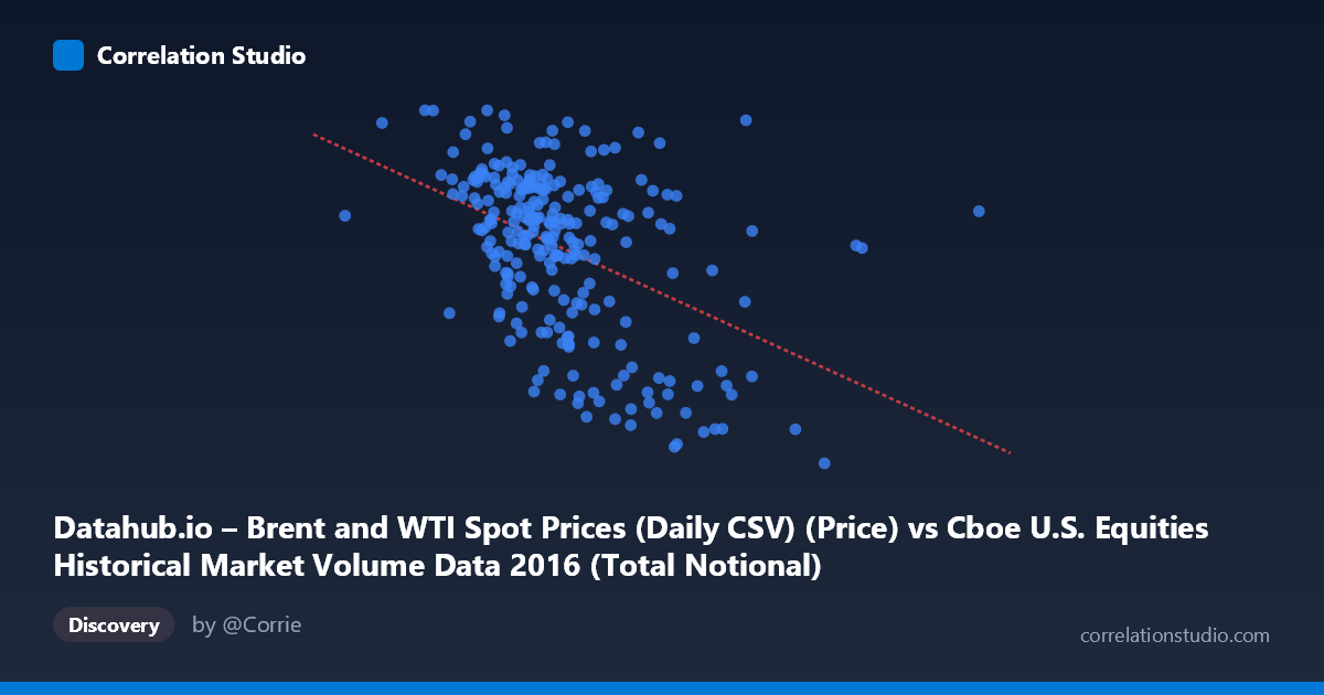
Datahub.io – Brent and WTI Spot Prices (Daily CSV) (Price) vs Cboe U.S. Equities Historical Market Volume Data 2016 (Total Notional)
- Pearson correlation (r)
- -0.4521
- Spearman correlation
- -0.4455
- p-value
- 0
- Sample size (n)
- 251
- 95% confidence interval
- -0.5454 to -0.3478
- Granger causality
- None
- Granger optimal lag
- 1
AI analysis
Analysis: Brent Crude Oil Prices vs. U.S. Equity Market Notional Volume (2016)
Relationship Overview The scatterplot reveals a moderate negative relationship between U.S. equity market total notional trading volume (X-axis) and Brent crude oil spot prices (Y-axis) across 2016. As daily equity market notional volume increases, Brent crude prices tend to decrease. The linear regression equation (y = -7.13×10⁻¹⁰x + 57.23) confirms this inverse slope, suggesting that on days with exceptionally high equity trading volume, oil prices tend to be lower. Visually, the data forms a broadly dispersed cloud with a discernible downward trend, though substantial scatter around the regression line is immediately apparent, indicating the relationship is real but far from deterministic.
Correlation Strength and Statistical Significance The Pearson correlation of r = -0.452 indicates a moderate negative association, but the explanatory power is modest: R² = 0.204, meaning only about 20.4% of the variance in Brent crude prices is explained by equity notional volume. The remaining ~80% of price variation is driven by factors entirely outside this model. The 95% confidence interval of [-0.545, -0.348] is meaningfully negative throughout — it does not straddle zero — lending credibility to the direction of the effect. The p-value of 4.75×10⁻¹⁴ is extraordinarily small, confirming the correlation is highly unlikely to be a chance artifact given n = 251 paired observations drawn from a population of N = 3,622. However, statistical significance here is partly a function of sample size; practical significance remains limited given the modest R². Critically, Granger causality tests find no significant predictive direction in either direction (X→Y: F = 0.41, p = 0.52; Y→X: F = 0.20, p = 0.65), meaning neither variable reliably predicts the other's future values at a one-period lag. The correlation is contemporaneous and associative, not temporally predictive.
Notable Patterns, Clusters, and Outliers Several structural features stand out in the data. The bulk of observations cluster in the notional volume range of roughly 14–22 billion, with oil prices concentrated between 40–54 USD/barrel, forming a reasonably dense core. However, there is a distinct sparse tail of high-volume outliers extending toward 25–40 billion in notional value, and these points almost uniformly correspond to low oil prices (26–34 USD/barrel) — most strikingly, the point at approximately (32.8B, 26.01) sits in isolation as the most extreme outlier in both dimensions. This cluster of high-volume/low-price days likely corresponds to the volatile early-2016 period when oil prices briefly collapsed to multi-year lows and equity market stress drove elevated trading volumes. Conversely, the lower-left region (low volume, higher oil prices ~48–54) represents the more stable mid-to-late 2016 trading environment. The relationship appears to be driven substantially by these tail observations, raising questions about whether the correlation holds uniformly across the full distribution.
Confounding Factors and Caveats Several important caveats apply. First, reverse causality and common-cause confounding are plausible: both variables could be jointly responding to macroeconomic shocks (e.g., Federal Reserve policy signals, geopolitical events, China growth fears in early 2016) rather than one influencing the other. Second, elevated equity notional volume on stressed days reflects fear and volatility rather than directional market sentiment, which may mechanically co-occur with commodity sell-offs — the VIX or market volatility index is a likely omitted variable. Third, the year 2016 was atypically eventful (oil price collapse in January, Brexit in June, U.S. election in November), meaning this correlation may not generalize to other periods. Fourth, the column label assignments appear somewhat counterintuitive — the X-axis is labeled as oil price data but represents equity volume, and the Y-axis represents Brent prices — warranting verification of dataset column mapping before drawing firm conclusions. Finally, the Granger test uses only a lag of 1 period, and longer lags might reveal delayed predictive relationships.
Actionable Insights and Further Investigation Practitioners should treat this correlation as a signal worth monitoring but not a reliable trading or forecasting rule — with only 20% of variance explained and no Granger causality, the relationship cannot support directional predictions. Further investigation should include: (1) incorporating the VIX or realized volatility as a control variable to test whether the correlation persists after accounting for market stress; (2) segmenting the data by quarter or market regime (e.g., pre/post-Brexit, pre/post-election) to test whether the correlation is driven by specific episodes; (3) extending Granger causality tests to lags of 2–5 periods and using a VAR framework with control variables; and (4) replicating this analysis across multiple years to assess whether 2016 represents a structural relationship or an anomalous co-movement. The isolation of the extreme high-volume/low-price cluster for separate analysis would also clarify whether the correlation is regime-dependent.
X dataset: Cboe U.S. Equities Historical Market Volume Data 2016
Y dataset: Datahub.io – Brent and WTI Spot Prices (Daily CSV)
Part of experiment: Daily - Cboe U.S. Equities Historical Market Volume Data 2016 vs Datahub.io – Brent and WTI Spot Prices (Daily CSV)