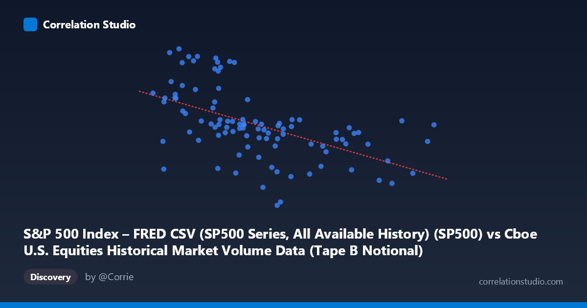
S&P 500 Index – FRED CSV (SP500 Series, All Available History) (SP500) vs Cboe U.S. Equities Historical Market Volume Data (Tape B Notional)
- Pearson correlation (r)
- -0.5397
- Spearman correlation
- -0.6197
- p-value
- 0
- Sample size (n)
- 98
- 95% confidence interval
- -0.6667 to -0.3822
- Granger causality
- None
- Granger optimal lag
- 10
AI analysis
Scatterplot Analysis: S&P 500 Index vs. Cboe Tape B Notional Volume
Relationship Overview The scatterplot reveals a negative relationship between the S&P 500 Index level and Cboe Tape B Notional Volume, captured by the regression equation y = -4.28×10⁻⁸x + 7,463.1. As the S&P 500 rises (X ranging from ~7.1B to ~21.0B index units), Tape B Notional Volume tends to decline (Y ranging from ~6,344 to ~7,501). This is an intuitively interesting inverse pattern: higher equity valuations are associated with lower notional trading volume on Tape B exchanges, suggesting that bull market conditions may coincide with reduced trading urgency or liquidity rotation away from Tape B securities (typically NYSE American/regional exchange-listed stocks).
Correlation Strength and Statistical Significance The Pearson correlation of r = -0.5397 indicates a moderate negative association, but the explanatory power is more modest than the headline number suggests: R² = 0.2913, meaning only 29.1% of the variance in Tape B Notional Volume is explained by the S&P 500 level. The remaining ~71% is driven by factors not captured in this bivariate model. The 95% confidence interval of [-0.667, -0.382] is entirely negative, confirming directional consistency, and the p-value of 9.78×10⁻⁹ makes this correlation highly statistically significant given n = 98 paired samples drawn from a population of N = 1,980. However, the Granger causality tests yield no significant predictive directionality in either direction (X→Y: F = 0.856, p = 0.578; Y→X: F = 1.037, p = 0.423) at the optimal 10-period lag. This is a critical caveat: while the variables co-move statistically, neither reliably predicts the other in a temporal sequence, meaning the correlation is likely driven by a shared underlying factor rather than a causal mechanism.
Notable Patterns, Clusters, and Outliers Several features stand out in the data. There is a moderate scatter cloud concentrated between S&P values of ~9B–14B and Tape B Notional of ~6,800–7,100, forming the densest cluster. At lower S&P levels (~7.1B–9.5B), Tape B Notional values cluster noticeably higher (7,100–7,501), consistent with the negative trend. At higher S&P levels (17B), values spread more widely but generally trend lower. Notable outliers include: (13,400,251,082; 6,368.85) and (13,233,916,266; 6,343.72) — both showing anomalously low Tape B Notional at mid-range S&P levels — and (8,390,501,362; 7,501.24) and (7,932,262,077; 7,473.47), which sit at the high-volume extreme. The outliers at mid-range X values that show very low Y values (the ~6,344–6,370 floor) suggest episodic volume suppression events unrelated to market level. The relationship also appears to show slight non-linearity, with a potentially steeper decline at lower S&P values that flattens somewhat at high values, hinting at a possible logarithmic or threshold relationship.
Confounding Factors and Interpretation Caveats Several important caveats limit causal interpretation. First, the dataset labels appear to be swapped in metadata: the X-axis is labeled as coming from the Cboe market volume dataset but described as "S&P 500 Index – FRED CSV," and vice versa — this warrants verification before drawing firm conclusions. Second, the time window (January–May 2026, ~98 trading days) is narrow, and both series are highly sensitive to macro regime changes, earnings seasons, and volatility events that compress this short window. Third, Tape B Notional is influenced by factors entirely independent of market level: exchange fee changes, market maker behavior, ETF rebalancing cycles, and seasonal trading patterns. Fourth, the S&P 500 itself could be functioning as a proxy for market volatility or risk appetite, with the true driver being VIX or macro uncertainty rather than price level per se. The lack of Granger causality reinforces that a common driver — perhaps macroeconomic conditions or investor sentiment — is likely responsible for the observed co-movement.
Actionable Insights and Further Investigation Given the moderate correlation and lack of Granger causality, practitioners should avoid using S&P 500 level alone as a predictor of Tape B trading volume. Instead, a more robust model should incorporate volatility measures (VIX), market breadth indicators, and Tape A/C volumes as controls to isolate Tape B-specific dynamics. It would be valuable to extend the time series beyond the 5-month window to test whether this negative relationship holds across full market cycles, including bear markets and recovery phases. Investigating the two low-volume outliers (~6,344 and ~6,369) for specific dates could reveal calendar effects or structural market events worth flagging. Finally, a multivariate regression or machine learning approach including lagged variables, volatility regimes, and macroeconomic indicators would likely substantially improve on the 29.1% variance explained and provide more actionable trading or risk management insights.
X dataset: Cboe U.S. Equities Historical Market Volume Data
Y dataset: S&P 500 Index – FRED CSV (SP500 Series, All Available History)
Part of experiment: Daily - Cboe U.S. Equities Historical Market Volume Data vs S&P 500 Index – FRED CSV (SP500 Series, All Available History)