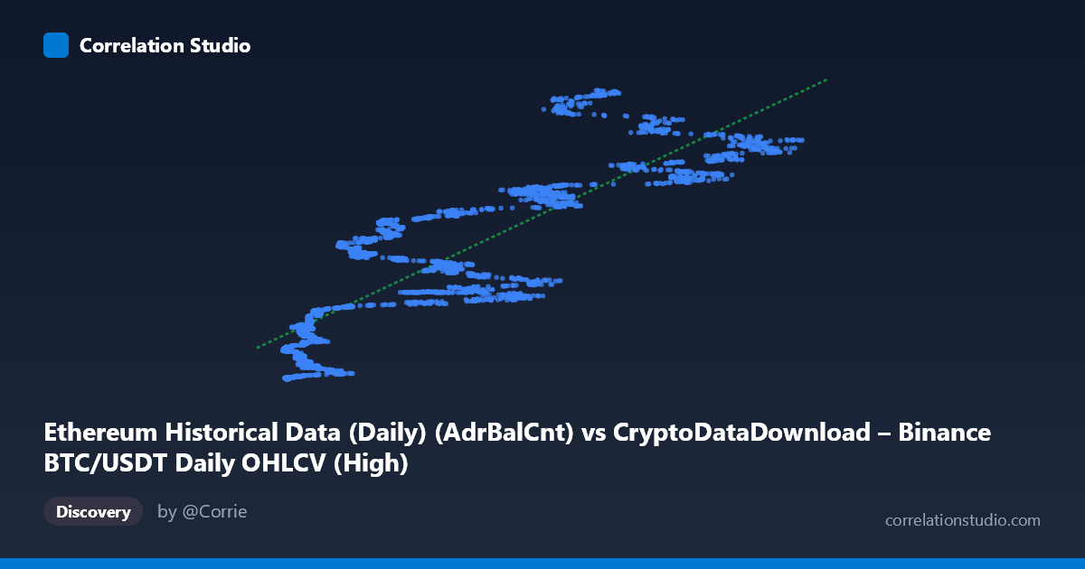
Ethereum Historical Data (Daily) (AdrBalCnt) vs CryptoDataDownload – Binance BTC/USDT Daily OHLCV (High)
- Pearson correlation (r)
- 0.8564
- Spearman correlation
- 0.8859
- p-value
- 0
- Sample size (n)
- 3191
- 95% confidence interval
- 0.8469 to 0.8654
- Granger causality
- None
- Granger optimal lag
- 10
- Time coverage
- 2017-08-17 to 2026-05-20
AI analysis
Analysis: Ethereum Address Count (AdrBalCnt) vs. Binance BTC/USDT Daily High
1. What the Visualization Reveals
The scatterplot shows a strong, positive, generally monotonic relationship between the X variable (labeled as Ethereum "AdrBalCnt" but drawn from BTC/USDT OHLCV metadata — see caveats below) and Y (BTC/USDT daily high price). As X increases from roughly 3,300 to 126,000, Y rises from under $3M to nearly $193M, tracking the fitted line y = 1306.48x + 27.2M reasonably well but with substantial scatter, especially in the mid-range (X ≈ 20,000–70,000), where Y values for similar X can span tens of millions of dollars (e.g., X≈28,000 yields Y values from ~52M to ~108M across different sample points).
2. Strength, Direction, and Predictive Direction
The correlation (r = 0.8564) is strong and positive, with r² = 0.7334 indicating that 73.3% of the variance in Y is explained by X in a simple linear model — leaving roughly 27% unexplained, which is non-trivial given the visible spread in the mid-density region. The 95% CI [0.8469, 0.8654] is tight, and p ≈ 0 confirms this correlation is highly statistically significant and not a product of sampling noise, largely a function of the large N (3,191). However, statistical significance here should not be conflated with practical precision for point-prediction — the residual scatter is meaningful. Critically, the Granger causality tests show no significant predictive direction in either direction (X→Y: p=0.384; Y→X: p=0.155) at the optimal lag of 10 periods. This means that despite the strong contemporaneous correlation, neither series reliably forecasts the other's future movements — the relationship is likely driven by a shared underlying trend (e.g., both series trending upward over 2017–2026) rather than one causing or leading the other.
3. Notable Patterns and Features
The relationship appears to flatten or show heteroscedasticity at higher X values (80,000), where Y values cluster more tightly in the 140M–190M range, suggesting possible saturation or ceiling effects. Conversely, at low X (<15,000), Y values are tightly clustered near the origin (under 50M), indicating a cleaner, more linear relationship in this lower regime. The mid-range (20,000–70,000) shows the greatest vertical dispersion, hinting at a possible regime change, structural break, or the influence of a third factor (like time/market cycle) that isn't captured in the two-variable scatter. There's no evidence of multiple discrete clusters, but the variance pattern suggests a possible logarithmic or power-law relationship might fit better than a strict linear one.
4. Confounding Factors and Caveats
The metadata is confusing and should be flagged: X is labeled as an Ethereum on-chain metric (active address balance count) but the axis header cites "CryptoDataDownload – Binance BTC/USDT Daily OHLCV," while Y is BTC/USDT price data labeled under an Ethereum dataset. This mismatch suggests possible mislabeling in the data pipeline — the "relationship" may actually be between an Ethereum network metric and Bitcoin price, or the labels are swapped entirely. This matters immensely for interpretation: correlating an ETH address count with BTC price is a cross-asset relationship likely driven by common crypto-market-wide bull/bear cycles (2017–2026 covers multiple major cycles), not a direct causal mechanism. Both series are also likely non-stationary (trending) time series, which is a classic driver of spurious correlation — this alone could explain the high r despite the lack of Granger causality, since trending series often show strong correlation without any lead-lag predictive relationship.
5. Actionable Insights and Suggestions
1. Verify data labeling — confirm which asset/metric is actually on each axis before drawing further conclusions; the current labels are internally inconsistent. 2. Test stationarity (ADF/KPSS tests) and consider differencing or working with returns/growth rates rather than levels to check whether the correlation persists or vanishes (common with trending crypto series). 3. Segment by time period/market cycle (bull vs. bear phases) to see if the relationship holds consistently or is driven by specific eras (e.g., 2020–2021 bull run). 4. Explore non-linear fits (log-log or polynomial) given the apparent flattening at high X and fan-shaped residuals at mid-range X. 5. Given the null Granger result, avoid using this relationship for trading or forecasting purposes — the correlation is descriptive/contemporaneous, not predictive.
X dataset: CryptoDataDownload – Binance BTC/USDT Daily OHLCV
Y dataset: Ethereum Historical Data (Daily)
Part of experiment: Bitcoin - CryptoDataDownload – Binance BTC/USDT Daily OHLCV vs Ethereum Historical Data (Daily)