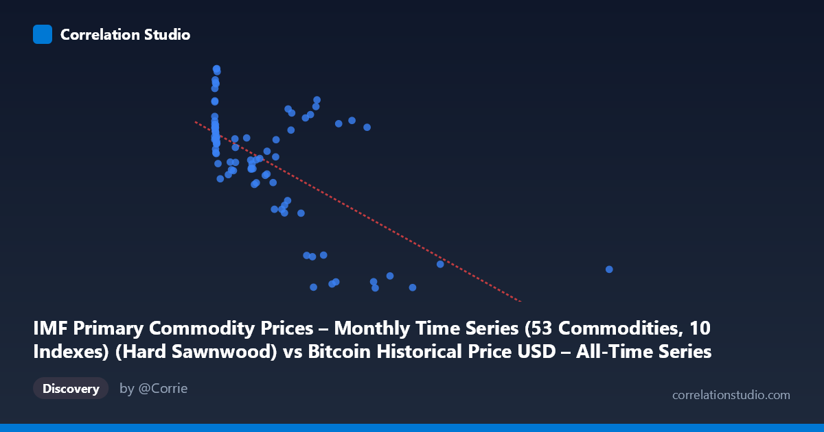
IMF Primary Commodity Prices – Monthly Time Series (53 Commodities, 10 Indexes) (Hard Sawnwood) vs Bitcoin Historical Price USD – All-Time Series (Habrador) (Price)
- Pearson correlation (r)
- -0.6377
- Spearman correlation
- -0.5409
- p-value
- 0
- Sample size (n)
- 83
- 95% confidence interval
- -0.7502 to -0.4893
- Granger causality
- None
- Granger optimal lag
- 10
- Time coverage
- 2010-08-01 to 2017-06-01
AI analysis
Analysis: Hard Sawnwood Prices vs. Bitcoin Price
1. Relationship Overview
The scatterplot shows a moderate negative relationship between hard sawnwood commodity prices (X-axis) and Bitcoin price (Y-axis). The data reveals a distinctive pattern: a dense cluster of points at low X-values (roughly 0–700) spanning the full range of Y-values (670–975), followed by a sparser tail of higher X-values that correspond almost exclusively to lower Y-values (670–900). This creates the visual impression of a downward-sloping trend, though it's driven substantially by the distribution shape rather than a tight linear coupling throughout.
2. Strength, Direction, and Statistical Confidence
The correlation coefficient (r = -0.638) indicates a moderate negative linear relationship, with R² = 0.407 meaning sawnwood prices statistically explain about 41% of the variance in Bitcoin price — leaving the majority (59%) unexplained by this single variable. The 95% CI [-0.750, -0.489] is reasonably tight and entirely negative, and the p-value (9×10⁻¹¹) confirms the correlation is highly unlikely to be due to chance. However, the Granger causality tests (both directions non-significant, p 0.20) indicate that neither variable helps predict future values of the other beyond their own historical patterns. This is a critical distinction: the relationship is associative, not predictive — sawnwood prices don't lead Bitcoin price movements (or vice versa) in a temporal/causal sense, despite the contemporaneous statistical correlation.
3. Notable Patterns and Outliers
Several features stand out: - Bimodal Y-clustering: Bitcoin prices cluster around two bands — roughly 780–975 (a "high" regime) and 670–720 (a "low" regime) — suggesting the relationship may reflect distinct time periods or market regimes rather than a smooth continuous trend. - Sparse high-X tail: Points beyond X=700 (up to X=2452) all fall in the lower Y-band (670–900), which likely has outsized leverage on the regression slope despite representing few observations. - Dense low-X cluster: The majority of points sit at X<50 with high variance in Y, suggesting sawnwood price alone is a poor predictor within this range.
4. Confounding Factors and Caveats
This pairing is a spurious-correlation candidate: sawnwood commodity prices and Bitcoin price have no plausible direct economic linkage. Both are more likely driven by shared macro factors — broad risk sentiment, US dollar strength, global liquidity/interest rate cycles, or simply the fact that both series trend over the 2010–2017 window (Bitcoin's early exponential rise, commodity supercycle dynamics post-2011). Time-series data like this often exhibit "nonsense regression" due to trending/non-stationary series inflating r² artificially. Additionally, n=83 paired points sampled from a population of 449 raises questions about sampling method and whether monthly alignment/interpolation between differently-frequency datasets biases results.
5. Suggestions for Further Investigation
- Test for stationarity (ADF test) on both series; if non-stationary, difference the data and recheck correlation to rule out spurious trend-driven correlation. - Control for time/macro variables (e.g., USD index, S&P 500, gold) via partial correlation or multivariate regression to see if the sawnwood-BTC link survives. - Segment by regime (pre-2013 vs. post-2013 Bitcoin bull runs) to check if correlation is period-specific rather than structural. - Given the lack of Granger causality, avoid using sawnwood prices as a predictive signal for Bitcoin trading models; treat the correlation as descriptive/historical rather than actionable for forecasting.
X dataset: Bitcoin Historical Price USD – All-Time Series (Habrador)
Y dataset: IMF Primary Commodity Prices – Monthly Time Series (53 Commodities, 10 Indexes)
Part of experiment: Bitcoin - Bitcoin Historical Price USD – All-Time Series (Habrador) vs IMF Primary Commodity Prices – Monthly Time Series (53 Commodities, 10 Indexes)