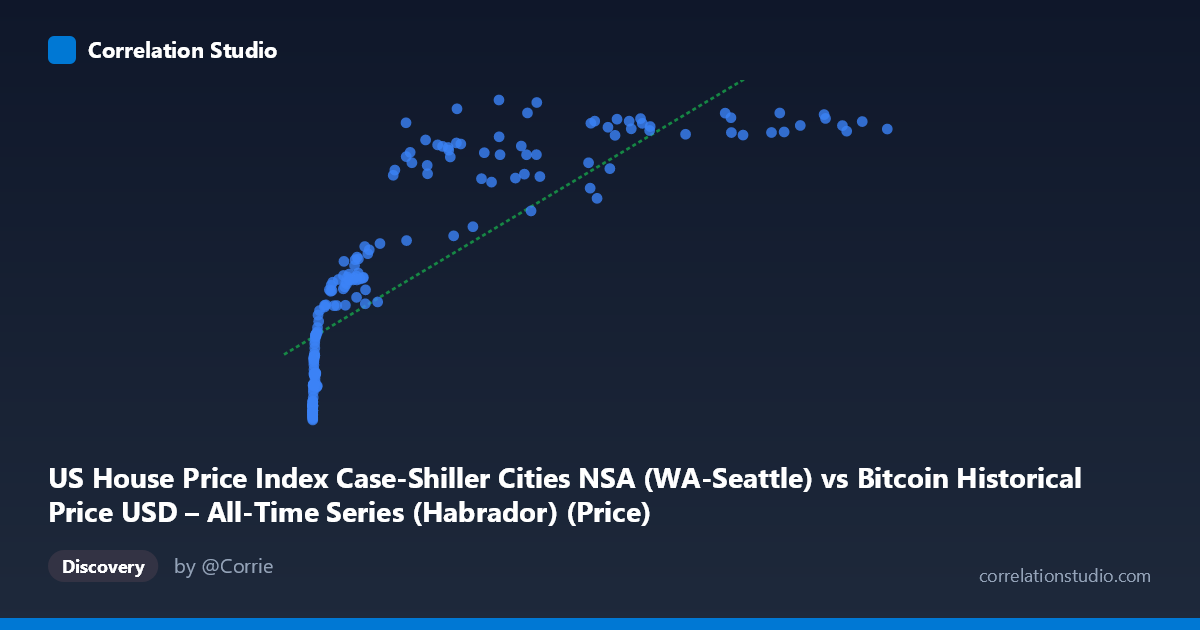
US House Price Index Case-Shiller Cities NSA (WA-Seattle) vs Bitcoin Historical Price USD – All-Time Series (Habrador) (Price)
- Pearson correlation (r)
- 0.8177
- Spearman correlation
- 0.9638
- p-value
- 0
- Sample size (n)
- 189
- 95% confidence interval
- 0.7641 to 0.86
- Granger causality
- None
- Granger optimal lag
- 9
- Time coverage
- 2010-08-01 to 2026-04-01
- Recomputed on refreshed data
- 2026-10-20 (r was 0.8133)
AI analysis
Analysis: Bitcoin Price vs. Seattle Case-Shiller Home Price Index
1. Relationship Overview
The scatterplot shows a strong positive association between Bitcoin's historical USD price and the Seattle Case-Shiller Home Price Index, but the relationship is clearly non-linear. At low Bitcoin values (under ~$1,000, the vast majority of data points), the Seattle index climbs steeply from ~130 to ~230, then the curve flattens considerably as Bitcoin prices scale into the tens of thousands. This produces a classic logarithmic or power-law shape rather than a straight line — a small increase in home prices corresponds to Bitcoin moving from cents to hundreds of dollars, while later, home prices barely move even as Bitcoin surges past $100,000.
2. Strength, Direction, and Statistical Confidence
The Pearson correlation (r = 0.813, r² = 0.661) indicates that a linear model explains about 66% of the variance in Y — a moderately strong fit, but the note that Spearman's ρ exceeds Pearson's r confirms the underlying relationship is monotonic but curved, meaning a log or polynomial transform of X would likely explain meaningfully more variance than the linear model does. The 95% CI [0.758, 0.859] is fairly tight and excludes zero, and the p-value (~0) confirms this correlation is not due to chance. However, Granger causality tests show no significant predictive direction in either direction (X→Y: p=0.51; Y→X: p=0.79) even at an optimal lag of 9 periods. This is a critical caveat: despite the strong contemporaneous correlation, neither series helps forecast the other's future values — the relationship is likely driven by a shared underlying trend (e.g., both series rising over calendar time) rather than genuine causal or lead-lag dynamics.
3. Notable Patterns and Outliers
The data is heavily right-skewed in X (mean 20,037 vs. median likely far lower, stdev 29,663), with the bulk of observations clustered at very low Bitcoin prices (sub-$1,000) corresponding to home index values in the 130–260 range — this is the steep "early" segment. A sparser but visible cluster exists at high Bitcoin prices ($40,000) where the home index plateaus around 350–400, showing diminishing marginal association. Some scatter/noise appears in the mid-range (e.g., prices around 27,000–45,000 showing index values from 293 to 402), suggesting other factors modulate Y once Bitcoin is in this range. No extreme bivariate outliers stand out, but the compression at high X values suggests a ceiling effect in the home price index that Bitcoin's continued growth doesn't track.
4. Confounding Factors and Caveats
Both variables are time series that have generally trended upward over the 2010–2026 window — Bitcoin due to adoption/speculation cycles, and Seattle home prices due to general inflation, wage growth, and housing demand. This shared secular trend is a classic confounding structure: two unrelated variables can appear strongly correlated simply because both increase with time (spurious correlation via a common "time" driver). The lack of Granger causality reinforces that this is likely coincidental trending rather than a causal economic link. Additionally, Bitcoin's extreme volatility (multiple boom-bust cycles) contrasts with the relatively smooth, seasonal nature of home price indices, meaning the linear model may be overstating the practical relationship's utility, especially for prediction.
5. Recommendations for Further Investigation
Given the non-linear signal, refit using a log-transformed X (log(Bitcoin price)) or polynomial regression to better capture the curve and likely boost explained variance beyond 66%. To disentangle genuine linkage from shared time trends, analysts should detrend both series (e.g., using year-over-year growth rates or differencing) and re-run correlation/Granger tests on the detrended/stationary series — this is the standard approach to avoid spurious time-series correlation. Additionally, consider whether a third variable (e.g., overall US monetary policy, inflation, or a risk-asset sentiment index) might drive both series independently, and test for cointegration to determine if there's a meaningful long-run equilibrium relationship despite the absence of short-term Granger causality.
X dataset: Bitcoin Historical Price USD – All-Time Series (Habrador)
Y dataset: US House Price Index Case-Shiller Cities NSA
Part of experiment: Bitcoin - Bitcoin Historical Price USD – All-Time Series (Habrador) vs US House Price Index Case-Shiller Cities NSA