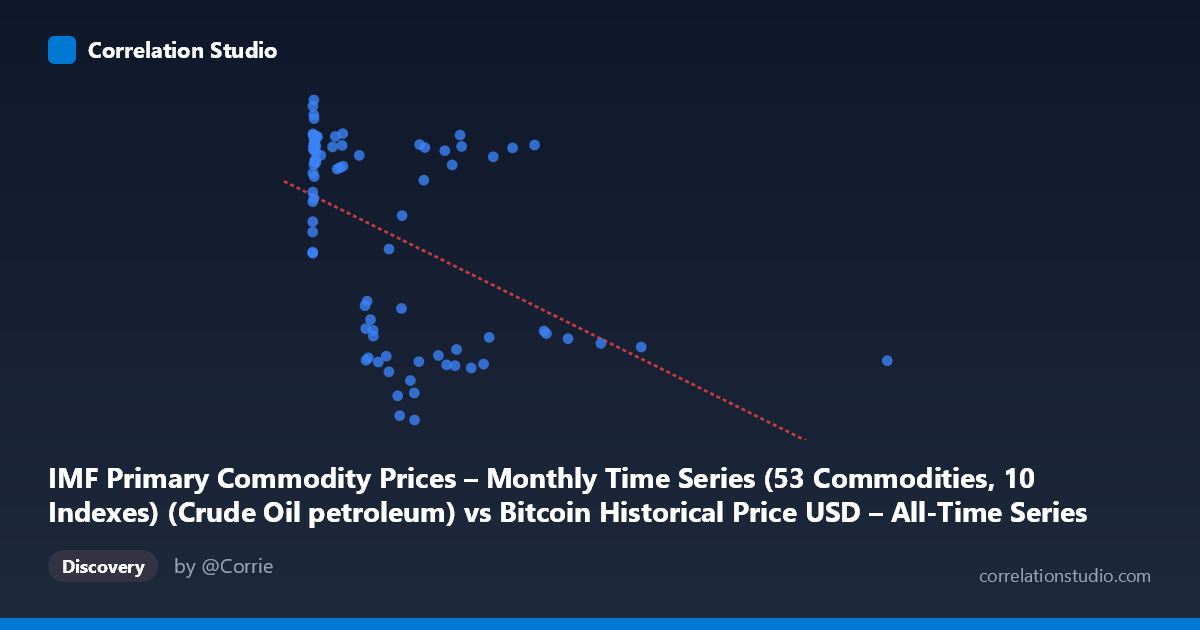
IMF Primary Commodity Prices – Monthly Time Series (53 Commodities, 10 Indexes) (Crude Oil petroleum) vs Bitcoin Historical Price USD – All-Time Series (Habrador) (Price)
- Pearson correlation (r)
- -0.4792
- Spearman correlation
- -0.4719
- p-value
- 0.000005
- Sample size (n)
- 83
- 95% confidence interval
- -0.6298 to -0.2938
- Granger causality
- None
- Granger optimal lag
- 8
- Time coverage
- 2010-08-01 to 2017-06-01
- Recomputed on refreshed data
- 2026-10-24 (r was -0.4792)
AI analysis
Analysis: Crude Oil Prices vs. Bitcoin Price
1. Overview of the Relationship
The scatterplot shows a moderate negative relationship between crude oil prices (X) and Bitcoin price (Y), though the pattern is far from a clean linear trend. A dense cluster of points sits at low X values (roughly 0–130, oil prices likely in normalized/index terms) where Y values span a wide range (from ~140 to ~222), indicating that when oil prices are low, Bitcoin prices show high variability rather than a tight relationship. As X increases beyond ~200, the Y values compress into a lower band (roughly 55–120), and this pattern holds fairly consistently out to the extreme X outlier at 2452.18 (Y=86.78).
2. Strength, Direction, and Statistical Confidence
The correlation coefficient (r = -0.479) indicates a moderate negative relationship, but r² = 0.230 reveals that only about 23% of the variance in Bitcoin price is explained by oil price movements — meaning roughly 77% of Bitcoin's price variation is driven by other factors entirely. The 95% CI [-0.630, -0.294] is reasonably tight and excludes zero, and the p-value (4.6e-06) confirms this negative association is statistically significant and not a product of chance in this sample. However, statistical significance should not be conflated with practical predictive power — with r² under 0.25, oil price alone is a weak standalone predictor of Bitcoin price. Critically, the Granger causality tests (p=0.249 for X→Y, p=0.167 for Y→X) show no significant temporal predictive direction in either direction — this is a contemporaneous/structural association, not a leading indicator relationship. This is an important distinction: the correlation may reflect shared macro exposure rather than one variable causally driving the other.
3. Patterns, Clusters, and Outliers
Two visually distinct regimes are apparent: a "low-X, high-and-variable-Y" cluster (X < 130, Y often 180–222) representing many observations clustered near the origin, and a "high-X, low-Y" tail (X 400, Y typically 55–115) extending to the extreme outlier at X=2452.18. This bimodal clustering — rather than a smooth linear cloud — suggests the relationship may be driven by two different market regimes or time periods (e.g., early Bitcoin history with low oil-index readings vs. later periods), rather than a continuous causal mechanism. The extreme X outlier (2452.18) sits within the expected low-Y band and doesn't appear to be an undue leverage point distorting the fit, but its presence should be checked via leverage/influence diagnostics (Cook's distance) since it's ~6x larger than the next-largest X values.
4. Confounding Factors and Caveats
Given the 2010–2017 time coverage, both series are non-stationary time series subject to strong trends, and the apparent negative correlation may be a spurious artifact of overlapping macro cycles (e.g., Bitcoin's early speculative rise coinciding with post-2014 oil price collapse) rather than genuine economic linkage. Neither series has been differenced or detrended here, so autocorrelation within each series likely inflates the apparent cross-correlation. Additionally, with n=83 sampled from a population of 449, there's potential sampling/aliasing bias, and monthly aggregation may mask higher-frequency dynamics. Common confounders (USD strength, global risk sentiment, interest rate regimes, regulatory shocks specific to Bitcoin) could independently affect both series without either causing the other.
5. Suggestions for Further Investigation
Analysts should re-run the correlation on detrended or differenced (% change) series to test whether the relationship survives after removing shared trend/non-stationarity — this is essential before drawing causal inferences. A regime-split analysis (pre-2014 vs. post-2014) would help clarify whether the bimodal clustering reflects distinct structural periods. Given the null Granger result, this relationship should be treated as descriptive/correlational only, not used for forecasting one series from the other. Expanding the analysis to include additional confounders (USD index, S&P 500, gold) in a multivariate framework would help isolate whether oil has any incremental explanatory power once broader macro conditions are controlled for.
X dataset: Bitcoin Historical Price USD – All-Time Series (Habrador)
Y dataset: IMF Primary Commodity Prices – Monthly Time Series (53 Commodities, 10 Indexes)
Part of experiment: Bitcoin - Bitcoin Historical Price USD – All-Time Series (Habrador) vs IMF Primary Commodity Prices – Monthly Time Series (53 Commodities, 10 Indexes)