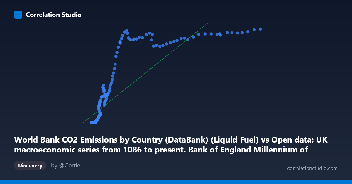
World Bank CO2 Emissions by Country (DataBank) (Liquid Fuel) vs Open data: UK macroeconomic series from 1086 to present. Bank of England Millennium of Macroeconomic Data. (Year) (value)
- Pearson correlation (r)
- 0.8416
- Spearman correlation
- 0.9583
- p-value
- 0
- Sample size (n)
- 266
- 95% confidence interval
- 0.8026 to 0.8735
- Granger causality
- Y → X
- Granger optimal lag
- 10
- Time coverage
- 1751-01-01 to 2016-01-01
AI analysis
Analysis: UK Macroeconomic Activity vs. CO₂ Liquid Fuel Emissions (1751–2016)
1. What the Visualization Reveals
The scatterplot depicts a broad positive relationship between UK macroeconomic output (Bank of England Millennium dataset values, plotted on the X-axis) and CO₂ emissions from liquid fuels (World Bank, Y-axis) across roughly 265 years of annual observations. The general sweep of the data traces a familiar development arc: low economic activity paired with near-zero liquid fuel emissions in the early historical period, rising through industrialization, and eventually reaching a plateau or saturation zone at high emission levels. Critically, a large cluster of points sits at Y ≈ 0 across a wide range of low-to-moderate X values, reflecting the pre-petroleum era when liquid fuels simply did not exist as an emissions source, regardless of economic scale.
2. Correlation Strength, Direction, and Causality
The Pearson correlation of r = 0.842 is strong, and the coefficient of determination R² = 0.708 means that approximately 70.8% of the variance in CO₂ liquid fuel emissions is statistically explained by the macroeconomic indicator — a substantial share for a relationship spanning two and a half centuries. The 95% confidence interval of [0.803, 0.874] is narrow and sits entirely above 0.80, confirming high precision in this estimate, and the p-value of effectively zero rules out chance. However, the Granger causality result is asymmetric and telling: Y Granger-causes X (F = 3.34, p = 0.0004) but X does not Granger-cause Y (F = 1.61, p = 0.104). This means past CO₂ liquid fuel emissions statistically predict future macroeconomic values with a 10-period lag, but not the reverse. This likely reflects the deep embedding of fossil-fuel energy consumption in economic productivity — energy use precedes or enables measurable economic output, rather than output mechanically driving emissions. This is an important directional nuance that a simple correlation would obscure.
3. Notable Patterns, Clusters, and Non-Linearity
Three structural features dominate the chart. First, a dense floor cluster at Y = 0 across X values roughly below ~20,000 represents the pre-liquid-fuel era; these points are not outliers in a statistical anomaly sense but a genuine regime boundary — liquid fuel combustion was zero because the technology did not exist. Second, a steep nonlinear ramp appears as X crosses roughly 20,000–50,000, where emissions jump rapidly from near-zero to several thousand units, consistent with the post-WWII motorization and petrochemical expansion. Third, the data exhibits clear saturation/plateau behavior at high X values (X 150,000), where Y asymptotes toward ~12,000–13,300, suggesting an emissions ceiling plausibly linked to efficiency improvements, fuel switching, or deindustrialization. The note that Spearman ρ exceeds Pearson r confirms what the eye detects: a logarithmic or sigmoid curve would fit substantially better than the fitted linear model y = 0.0411x + 883.92, which cannot capture the floor, ramp, and ceiling structure simultaneously.
4. Confounding Factors and Interpretive Caveats
Several confounds deserve caution. Temporal autocorrelation is severe — both series trend upward over centuries, meaning much of the correlation may reflect shared time trends rather than a direct causal economic-emissions mechanism (a classic spurious long-run correlation problem). Technology regime shifts (pre-petroleum, petroleum adoption, electrification, North Sea oil, service-sector transition) create structurally distinct sub-populations that the single regression line treats as homogeneous. The dataset join — merging a UK macroeconomic series with a World Bank country-level CO₂ series — raises questions about whether the CO₂ figures represent UK-only emissions or a broader aggregate, and whether the macroeconomic variable (GDP, wages, or another composite) is the most theoretically appropriate pairing. Finally, the 10-period Granger lag is long enough that confounding intermediate variables (energy prices, trade volumes, policy) almost certainly mediate the relationship.
5. Actionable Insights and Further Investigation
The saturation pattern above X ~ 150,000 is particularly actionable: it suggests that beyond a certain level of economic output, additional growth no longer drives proportional liquid fuel emissions — a potential empirical anchor for UK decarbonization policy analysis. Recommended next steps include: (a) fitting a logarithmic or piecewise regression to properly model the three regimes and obtain unbiased residuals; (b) segmenting the analysis by era (pre-1900, 1900–1970, 1970–2016) to test whether the relationship is stable or structurally shifting; (c) detrending both series (e.g., first-differencing or HP filter) before re-running Granger causality to eliminate spurious trend-driven results; (d) incorporating energy price data as a mediating variable to test whether the Granger signal from emissions to output runs through energy cost channels; and (e) cross-validating against other country datasets to determine whether this emissions-ceiling pattern is UK-specific or a general feature of post-industrial economies.
X dataset: Open data: UK macroeconomic series from 1086 to present. Bank of England Millennium of Macroeconomic Data. (Year)
Y dataset: World Bank CO2 Emissions by Country (DataBank)
Part of experiment: Yearly - Open data: UK macroeconomic series from 1086 to present. Bank of England Millennium of Macroeconomic Data. (Year) vs World Bank CO2 Emissions by Country (DataBank)