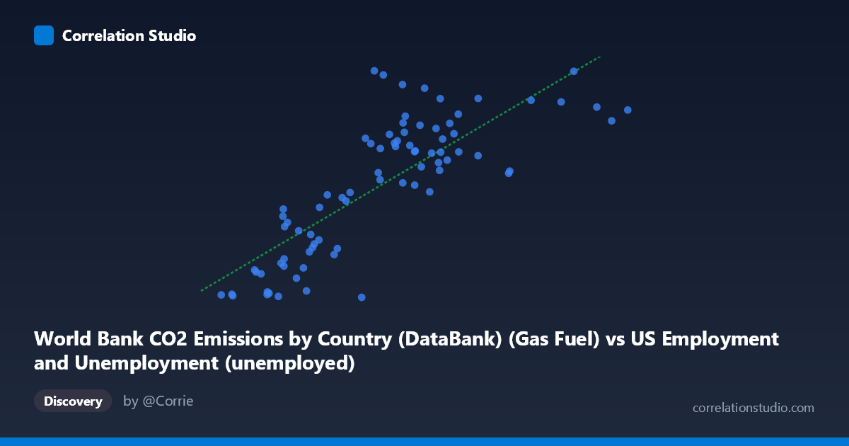
World Bank CO2 Emissions by Country (DataBank) (Gas Fuel) vs US Employment and Unemployment (unemployed)
- Pearson correlation (r)
- 0.8029
- Spearman correlation
- 0.8077
- p-value
- 0
- Sample size (n)
- 80
- 95% confidence interval
- 0.7081 to 0.8693
- Granger causality
- None
- Granger optimal lag
- 10
AI analysis
Scatterplot Analysis: Gas Fuel CO2 Emissions vs. US Unemployment
1. Overall Relationship
The scatterplot reveals a moderately strong positive relationship between World Bank gas fuel CO2 emissions and US unemployment figures across the 1941–2020 time period. As gas fuel emissions increase, unemployment tends to rise as well, though the relationship is far from deterministic. The linear regression equation (y = 1.217x + 1,161.25) suggests that for each unit increase in gas fuel CO2 emissions, unemployment increases by approximately 1.22 units. However, the wide vertical spread visible throughout the plot — particularly in the middle and upper ranges of X — makes clear that this is a noisy relationship with considerable unexplained variation at virtually every emission level.
2. Correlation Strength, Direction, and Causality
The Pearson correlation of r = 0.803 indicates a strong positive association, and the R² of 0.645 means that roughly 64.5% of the variance in unemployment is statistically explained by gas fuel emissions. While this is a substantial proportion, it also means that 35.5% of the variance remains unexplained, reminding us that the linear model is incomplete. The 95% confidence interval of [0.708, 0.869] is meaningfully narrow and excludes zero, and the p-value of effectively 0 confirms the correlation is highly statistically significant at any conventional threshold. Critically, however, Granger causality tests in both directions are non-significant (X→Y: F = 0.715, p = 0.706; Y→X: F = 0.931, p = 0.513), meaning neither variable reliably predicts the other in a temporally lagged sense, even at the optimal lag of 10 periods. This is a vital caveat: statistical correlation does not translate into temporal predictive power here, strongly suggesting the relationship is driven by a shared common trend rather than a direct causal mechanism.
3. Notable Patterns, Clusters, and Outliers
Several distinct features stand out in the data:
- A low-emission, low-unemployment cluster is visible in the lower-left region (X < ~3,000, Y < ~3,500), likely corresponding to the early decades of the dataset (1940s–1960s) when both emissions and the labor force were smaller. - A mid-range cluster around X = 6,000–9,000 shows substantial vertical scatter, with Y values ranging from roughly 8,000 to 16,000 — suggesting that similar emission levels coincide with very different unemployment outcomes, possibly reflecting economic cycles (recessions vs. expansions). - Notable outliers include the point near (6,001; 16,992), which sits far above the regression line and likely corresponds to a recession year with unusually high unemployment relative to emissions. Similarly, (5,560; 654) sits dramatically below the trend, indicating anomalously low unemployment at a moderate emissions level. - The upper-right cluster (X 12,000) appears to converge toward the regression line more tightly, suggesting a more consistent relationship at higher emission levels, possibly reflecting recent decades.
4. Confounding Factors and Interpretive Caveats
The most important caveat is that both variables are strongly driven by time — they are annual time-series from 1941 to 2020, and both gas fuel emissions and the absolute size of the US labor force (and thus unemployment counts) have generally grown over this 80-year period. This means the observed correlation almost certainly reflects a shared secular trend (population growth, economic expansion, industrialization) rather than any meaningful direct relationship between emissions and joblessness. The failure of Granger causality tests to detect directional predictability reinforces this interpretation. Additional confounders include: GDP growth (drives both emissions and employment), energy price shocks (oil crises affect both), structural economic shifts (deindustrialization reducing both manufacturing emissions and employment), and the fact that unemployment is measured in persons while emissions are measured in CO2 mass units — making the regression equation dimensionally and conceptually difficult to interpret directly. The dataset labels also suggest a possible cross-dataset join between US employment data and World Bank global emissions data, raising questions about geographic alignment.
5. Actionable Insights and Further Investigation
Given the spurious-trend concern, the most important next step would be to detrend both time series (e.g., first-differencing or removing a common time trend) and retest the correlation — it would likely diminish substantially. Researchers should also disaggregate by decade to test whether the correlation holds consistently across sub-periods or is driven entirely by long-run growth trends. Replacing absolute unemployment counts with the unemployment rate (%) would control for labor force size growth and provide a more meaningful variable. It would also be valuable to test against US-specific gas fuel CO2 emissions rather than a World Bank global figure, to ensure geographic comparability. Finally, incorporating GDP, energy prices, and recession indicators as control variables in a multivariate model would help isolate whether any residual relationship between emissions and unemployment persists after accounting for obvious confounders. The current correlation, while statistically robust, should not be interpreted as evidence of a meaningful policy-relevant link between gas fuel combustion and unemployment outcomes.
X dataset: US Employment and Unemployment
Y dataset: World Bank CO2 Emissions by Country (DataBank)
Part of experiment: Yearly - US Employment and Unemployment vs World Bank CO2 Emissions by Country (DataBank)