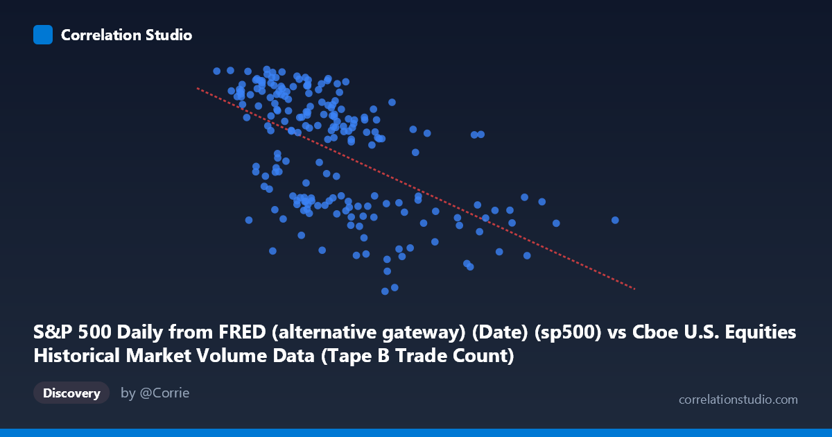
S&P 500 Daily from FRED (alternative gateway) (Date) (sp500) vs Cboe U.S. Equities Historical Market Volume Data (Tape B Trade Count)
- Pearson correlation (r)
- -0.5591
- Spearman correlation
- -0.5928
- p-value
- 0
- Sample size (n)
- 202
- 95% confidence interval
- -0.6472 to -0.4562
- Granger causality
- None
- Granger optimal lag
- 10
- Time coverage
- 2026-01-02 to 2026-10-21
- Recomputed on refreshed data
- 2026-10-23 (r was -0.5591)
AI analysis
Analysis: S&P 500 Index vs. Cboe Tape B Trade Count
Relationship Overview The scatterplot reveals a moderate negative relationship between the S&P 500 index level (X-axis) and Cboe U.S. Equities Tape B trade count (Y-axis) over the early 2026 period. The linear regression equation (y = −0.000442x + 7386.13) indicates that as the S&P 500 index rises, Tape B trade counts tend to decline. This is visually apparent in the downward-sloping trend, though with considerable scatter. The relationship is intuitive in one sense — rising equity markets may reduce urgency-driven or defensive trading activity, while market stress or downturns can spike trade volumes as participants react and rebalance.
Correlation Strength and Statistical Significance The correlation coefficient of r = −0.42 represents a moderate negative association, but the variance explained (r² = 0.176) tells a more sobering story: only 17.6% of the variability in Tape B trade counts is accounted for by S&P 500 levels. The remaining ~82% is driven by other factors entirely. The 95% confidence interval of [−0.57, −0.24] is meaningfully negative throughout — it does not cross zero — and the p-value of 1.7×10⁻⁵ confirms the relationship is highly statistically significant, making random chance an implausible explanation. However, statistical significance should not be conflated with practical magnitude; the effect size is modest. Critically, Granger causality tests reveal no significant temporal predictive relationship in either direction (X→Y: F = 0.92, p = 0.52; Y→X: F = 1.05, p = 0.41), meaning neither variable reliably predicts the other's future values at the optimal 10-period lag. This absence of Granger causality substantially limits any causal narrative.
Notable Patterns, Clusters, and Outliers The data exhibit a visible clustering of observations in the 750,000–1,100,000 range on the X-axis, corresponding to trade counts broadly between 6,800 and 7,500 — suggesting the majority of trading days occurred with the S&P 500 in a mid-range zone during this sample period. Several notable outliers are visible: points near (1,115,472, 6,369), (1,085,027, 6,344), and (1,352,971, 6,506) represent unusually low trade counts relative to the trend, potentially corresponding to low-volatility or holiday-adjacent sessions. Conversely, points near (769,704, 7,473), (823,636, 7,501), and (873,605, 7,446) show elevated trade counts at lower index levels. There is also heteroscedasticity apparent at lower X values — trade counts are much more dispersed when the index is lower, narrowing at higher index levels — suggesting the relationship is not uniformly linear across the full range.
Confounding Factors and Caveats Several important caveats apply. First, the dataset label descriptions appear swapped — Tape B Trade Count is listed as a column from the S&P 500 dataset and vice versa, warranting data provenance verification before drawing firm conclusions. Second, Tape B covers NYSE American and regional exchange listings, which may respond to sector-specific dynamics rather than broad market levels. Third, the sample window (January–May 2026) is narrow and may capture period-specific structural effects such as options expiration cycles, earnings seasons, or macro events that create spurious correlations. Fourth, market volume and trade counts are heavily influenced by algorithmic trading, market maker behavior, and exchange fee structures — none of which are captured by index level alone.
Actionable Insights and Further Investigation Given that only ~18% of variance is explained and Granger causality is absent, practitioners should avoid using S&P 500 level as a standalone predictor of Tape B activity. A more productive path would involve incorporating volatility measures (e.g., VIX), options expiration calendars, and time-of-month effects as additional regressors. Segmenting the data by day-of-week or earnings season could reveal whether the negative relationship is concentrated in specific contexts. It would also be valuable to compare Tape A and Tape C trade counts against the same index variable to determine whether the negative relationship is a Tape B phenomenon or a broader market-volume dynamic. Finally, extending the time series beyond five months would substantially improve the reliability of both the correlation estimate and the Granger causality tests, which currently suffer from limited lag resolution.
X dataset: Cboe U.S. Equities Historical Market Volume Data
Y dataset: S&P 500 Daily from FRED (alternative gateway) (Date)
Part of experiment: Daily - Cboe U.S. Equities Historical Market Volume Data vs S&P 500 Daily from FRED (alternative gateway) (Date)