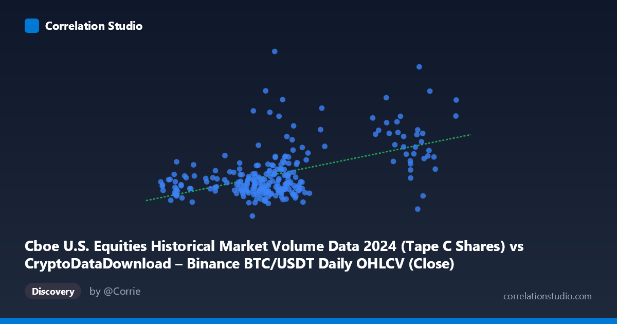
Cboe U.S. Equities Historical Market Volume Data 2024 (Tape C Shares) vs CryptoDataDownload – Binance BTC/USDT Daily OHLCV (Close)

Pearson correlation (r): 0.5148
Spearman correlation: 0.3865
p-value: 0
Sample size (n): 252
95% confidence interval: 0.4178 to 0.6002
Granger causality: None
Granger optimal lag: 10
Time coverage: 2024-01-02 to 2024-12-31

AI analysis

Analysis: Cboe Equities Volume vs. BTC/USDT Close Price

1. Relationship Overview

The scatterplot displays a moderate positive association between Cboe U.S. equities trading volume (Tape C shares) and Bitcoin's closing price on Binance. Note that despite the axis labels suggesting otherwise, based on the data ranges provided, the X-axis (39,568–106,133) actually represents the volume-like metric while Y (199M–658M) represents the price-scaled variable — the relationship shows a general upward drift, but with substantial scatter around the trend line.

2. Strength, Direction, and Statistical Confidence

The correlation coefficient (r = 0.5148) indicates a moderate positive relationship, but the r² of 0.265 reveals that only 26.5% of the variance in Y is explained by X — meaning nearly 75% of the movement in Bitcoin's price is driven by factors unrelated to this equities volume measure. The 95% confidence interval [0.418, 0.600] is reasonably tight and excludes zero, and the p-value (~0) confirms this correlation is statistically significant and not due to chance, given the sample size (n=252). However, statistical significance should not be conflated with practical predictive power — the relationship is real but weak enough that it offers limited standalone forecasting utility. Critically, the Granger causality tests show no significant predictive direction in either direction (X→Y: p=0.418; Y→X: p=0.390), even at an optimal lag of 10 periods. This is an important caveat: while the two series move together contemporaneously, neither reliably leads the other in time — the correlation appears to reflect a shared underlying driver or coincidental co-movement rather than a causal lead-lag relationship.

3. Notable Patterns and Outliers

The bulk of data clusters in the X-range of 55,000–72,000, with a secondary cluster around 95,000–101,000 — suggesting possible regime shifts or two distinct market periods (e.g., different volume regimes across the year). Within the main cluster, Y-values are highly dispersed (ranging roughly 200M–520M) for similar X-values around 60,000–70,000, indicating substantial noise/heteroscedasticity at lower X. A few notable outliers appear: one point near (64,144, 488M) and another near (67,024, 523M) sit well above the regression line, while (60,209, 199M) sits near the floor — these extreme Y-values at similar X levels underscore that X alone poorly constrains Y in the lower range. The second cluster (X 95,000) shows a tighter, somewhat elevated relationship, hinting at possible non-linearity or a level shift rather than a single continuous linear trend.

4. Confounding Factors and Caveats

Both series are time-based (2024 daily data), so they are likely both influenced by common macro factors — overall market risk sentiment, monetary policy announcements, seasonality, or liquidity conditions — rather than one directly driving the other. Equities volume and crypto pricing could be jointly responding to volatility events (e.g., Fed announcements, ETF news) without any direct mechanical link. Additionally, daily-level aggregation may mask intraday dynamics, and the lack of Granger causality suggests spurious or confounded correlation is a real possibility. Autocorrelation within each series (common in financial time series) can also inflate apparent correlation strength beyond genuine information content.

5. Suggestions for Further Investigation

Given the weak causal signal, analysts should treat this X variable as a coincident indicator at best, not a predictive one. Further work should: (a) test for a common third factor (e.g., VIX, overall market volume, macro liquidity indices) that might drive both series simultaneously; (b) explore non-linear or regime-switching models given the apparent two-cluster structure; (c) examine higher-frequency (intraday) data to check if causality emerges at shorter lags; and (d) apply cointegration tests (e.g., Engle-Granger) to determine if a long-run equilibrium relationship exists despite the absence of short-term Granger causality.

X dataset: CryptoDataDownload – Binance BTC/USDT Daily OHLCV

Y dataset: Cboe U.S. Equities Historical Market Volume Data 2024

Part of experiment: Bitcoin - CryptoDataDownload – Binance BTC/USDT Daily OHLCV vs Cboe U.S. Equities Historical Market Volume Data 2024