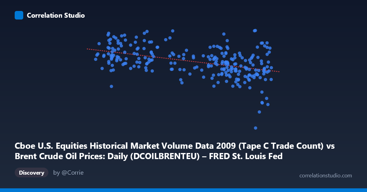
Cboe U.S. Equities Historical Market Volume Data 2009 (Tape C Trade Count) vs Brent Crude Oil Prices: Daily (DCOILBRENTEU) – FRED St. Louis Fed (DCOILBRENTEU)
- Pearson correlation (r)
- -0.445
- Spearman correlation
- -0.4451
- p-value
- 0
- Sample size (n)
- 252
- 95% confidence interval
- -0.539 to -0.3402
- Granger causality
- None
- Granger optimal lag
- 10
AI analysis
Scatterplot Analysis: Cboe Trade Count vs. Brent Crude Oil Price (2009)
Relationship Overview
The scatterplot reveals a moderate negative relationship between Cboe U.S. Equities tape C trade count (X-axis) and Brent Crude Oil daily spot prices (Y-axis) across 252 trading days in 2009. The linear regression equation (y = -3606.16x + 858,476) confirms that as equity trade counts increase, crude oil prices tend to decline. Visually, the data cloud slopes downward from left to right, though with considerable scatter throughout. This inverse relationship is intuitively interesting: higher equity market activity — potentially reflecting risk-off sentiment, volatility events, or institutional repositioning — appears loosely associated with lower oil prices, though the pattern is far from deterministic.
Correlation Strength and Statistical Significance
The Pearson correlation of r = -0.4450 indicates a moderate negative association, but the explanatory power is modest: R² = 0.1981, meaning only about 19.8% of the variance in oil prices is accounted for by trade volume counts. The remaining ~80% of price variation is driven by factors entirely outside this model. The 95% confidence interval of [-0.539, -0.340] is meaningfully below zero throughout, and the p-value of 1.16 × 10⁻¹³ confirms this is not a chance finding given the sample of 252 paired observations drawn from a population of 3,232. However, statistical significance here is substantially amplified by sample size — a moderate r with p < 0.001 should not be mistaken for a strong or practically meaningful relationship. Critically, Granger causality tests in both directions fail to reach significance (X→Y: F=1.34, p=0.21; Y→X: F=1.15, p=0.32), meaning neither variable reliably predicts the other temporally at the optimal 10-period lag. This rules out straightforward lead-lag predictive relationships and argues strongly against any causal interpretation.
Notable Patterns, Clusters, and Outliers
Several features stand out in the data distribution. There is a notable cluster of high trade-count observations (X 70) that spans a wide vertical range of oil prices (~$385K–$765K range in the Y metric), suggesting heteroscedasticity — variance in oil prices is not constant across trade volume levels. A prominent outlier at approximately (75.15, 185,887) sits dramatically below the regression line and the rest of the data cloud, likely representing an anomalous trading day and potentially exerting disproportionate influence on the regression slope. Similarly, a point near (56.63, 845,583) sits at the upper extreme of Y. On the lower-X end (X: 40–55), oil prices tend to cluster at higher levels with relatively less dispersion, while the higher-X region shows considerably more vertical spread — consistent with a funnel-shaped pattern that warrants formal heteroscedasticity testing.
Confounding Factors and Caveats
Several important caveats apply. First, the axis labels appear to be swapped in the dataset metadata — the X-axis is labeled as Brent crude price data while drawing from the Cboe volume dataset, and vice versa — suggesting a possible data labeling inconsistency that should be verified before drawing conclusions. Second, 2009 was an exceptional year characterized by the aftermath of the 2008 financial crisis, a historic equity market bottom in March, and a sharp oil price recovery from sub-$40 to near-$80 per barrel — making temporal autocorrelation and trend confounding a serious concern. Both series likely share a common driver (macroeconomic recovery trajectory) that creates spurious co-movement. Third, trade count on Tape C (NYSE Arca) reflects a subset of total market activity and may not represent broad equity market sentiment adequately. Finally, the non-Gaussian distribution of both variables and potential non-linearity in the relationship means Pearson r may not fully capture the true association structure.
Actionable Insights and Further Investigation
Given that Granger causality is absent and R² explains less than 20% of variance, this correlation should not be used for predictive modeling in its current form. Several next steps would strengthen the analysis: (1) Remove or winsorize the extreme outlier near (75.15, 185,887) and re-examine whether it structurally alters the regression; (2) Detrend both series to remove the shared 2009 macroeconomic recovery trend before computing correlation, which would isolate genuine co-movement from common trend contamination; (3) Test for non-linear relationships (e.g., polynomial or spline regression) given the apparent heteroscedasticity; (4) introduce control variables such as the VIX volatility index, USD index, or S&P 500 returns to partial out confounders; and (5) extend the analysis across multiple years to determine whether this negative relationship is stable or specific to the anomalous 2009 market environment.
X dataset: Brent Crude Oil Prices: Daily (DCOILBRENTEU) – FRED St. Louis Fed
Y dataset: Cboe U.S. Equities Historical Market Volume Data 2009
Part of experiment: Daily - Brent Crude Oil Prices: Daily (DCOILBRENTEU) – FRED St. Louis Fed vs Cboe U.S. Equities Historical Market Volume Data 2009