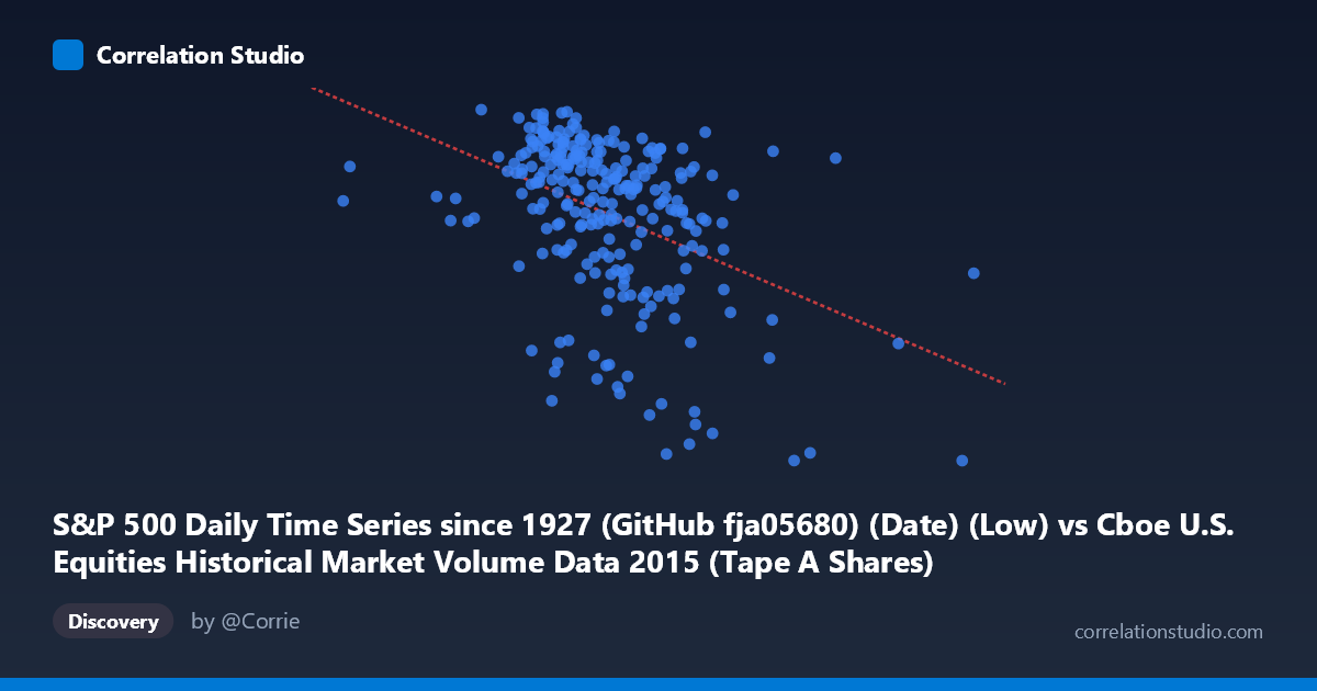
S&P 500 Daily Time Series since 1927 (GitHub fja05680) (Date) (Low) vs Cboe U.S. Equities Historical Market Volume Data 2015 (Tape A Shares)
- Pearson correlation (r)
- -0.4202
- Spearman correlation
- -0.4223
- p-value
- 0
- Sample size (n)
- 252
- 95% confidence interval
- -0.5169 to -0.3128
- Granger causality
- None
- Granger optimal lag
- 2
AI analysis
Analysis: S&P 500 Daily Low vs. Cboe Tape A Shares Volume (2015)
1. Overall Relationship The scatterplot reveals a moderate negative relationship between the S&P 500 daily low price (X-axis) and Cboe Tape A shares volume (Y-axis) across 252 trading days in 2015. As the S&P 500 daily low increases — indicating higher index price levels — Tape A share volume tends to decrease. This inverse pattern is consistent with well-documented market microstructure behavior: elevated equity prices often coincide with calmer, lower-volatility market regimes that attract less frenetic trading activity, while lower price levels frequently accompany heightened uncertainty and elevated turnover.
2. Correlation Strength, Direction, and Causality The Pearson correlation of r = −0.42 indicates a moderate negative association, but the explanatory power is modest: r² = 0.1765, meaning only about 17.7% of the variance in Tape A volume is explained by the S&P 500 daily low. The remaining ~82% is attributable to other factors. The 95% confidence interval of [−0.517, −0.313] is entirely negative and comfortably excludes zero, and the p-value of 3.36×10⁻¹² confirms this relationship is highly statistically significant — far beyond conventional thresholds — given the sample of 252 paired observations drawn from a population of 3,302. The linear regression equation (y = −4.86×10⁻⁷x + 2185.36) quantifies this: each one-unit increase in the daily low is associated with a decrease of roughly 0.000000486 in Tape A shares. Despite statistical significance, Granger causality tests yield no significant directional predictive relationship in either direction (X→Y: F=1.28, p=0.28; Y→X: F=0.55, p=0.58), meaning neither variable reliably predicts the other's future values at a 2-period lag. The correlation reflects contemporaneous co-movement, not a temporal lead-lag dynamic suitable for forecasting.
3. Notable Patterns, Clusters, and Outliers The scatterplot shows a discernible downward-sloping cloud with notable dispersion, suggesting the relationship is real but noisy. Several features stand out: - A dense cluster around X ≈ 230M–290M and Y ≈ 2040–2130 represents the majority of typical trading days, where the index remained in a relatively bounded range with moderate volume. - High-volume outliers at lower price levels — particularly points near X ≈ 108M–200M with Y values around 2060–2126 — suggest episodes where the index traded at unusually depressed intraday lows coinciding with elevated volume, consistent with sharp sell-offs or high-volatility events in mid-2015. - Low-volume readings at higher price levels (X 380M, Y < 1990) align with the August 2015 market correction period and its aftermath, where paradoxically some high-stress days may skew the pattern. - The point near (401M, 1867) is a notable outlier — the lowest Y value paired with one of the highest X values — potentially representing an anomalous or thinly traded session worth investigating independently.
4. Confounding Factors and Interpretive Caveats Several important caveats apply. Secular trends within 2015 — including the August correction and year-end drift — likely drive much of the correlation, meaning the relationship may be largely a manifestation of shared time-series trends rather than a structural economic link. Regime shifts (pre- vs. post-August correction) could create spurious correlation when pooled together. The datasets are also sourced from different primary datasets joined by date, introducing alignment risk and potential data provenance inconsistencies. Furthermore, Tape A specifically covers NYSE-listed securities, while the S&P 500 includes Nasdaq-listed names, creating a partial market overlap that limits direct comparability. Volume is also influenced by institutional calendar effects (quarter-ends, option expiration), seasonal liquidity patterns, and intraday reporting conventions not captured here.
5. Actionable Insights and Further Investigation Given that nearly 83% of volume variance remains unexplained, the following steps are recommended: - Segment the analysis by market regime (pre/post August 2015 correction) to test whether the correlation is stable or artifact of a specific stressed period. - Incorporate volatility measures (e.g., VIX) as a mediating variable — volatility likely explains both lower index levels and higher volume simultaneously, potentially reducing or eliminating the direct X→Y relationship. - Extend to multivariate regression, adding spread data, trade count, and notional value from the Cboe dataset to better characterize volume drivers. - Test alternative lags beyond 2 periods in Granger causality, as market microstructure effects may operate at daily or weekly scales not captured here. - Cross-validate with Tape B and C volume to assess whether the pattern is specific to NYSE-listed equities or broader across U.S. equity markets.
X dataset: Cboe U.S. Equities Historical Market Volume Data 2015
Y dataset: S&P 500 Daily Time Series since 1927 (GitHub fja05680) (Date)
Part of experiment: Daily - Cboe U.S. Equities Historical Market Volume Data 2015 vs S&P 500 Daily Time Series since 1927 (GitHub fja05680) (Date)