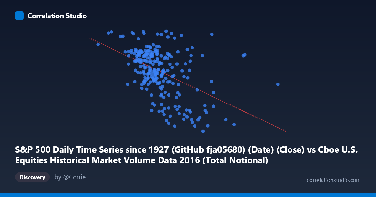
S&P 500 Daily Time Series since 1927 (GitHub fja05680) (Date) (Close) vs Cboe U.S. Equities Historical Market Volume Data 2016 (Total Notional)

Pearson correlation (r): -0.4757
Spearman correlation: -0.4655
p-value: 0
Sample size (n): 252
95% confidence interval: -0.566 to -0.3742
Granger causality: None
Granger optimal lag: 4

AI analysis

Analysis: S&P 500 Close Price vs. U.S. Equities Market Notional Volume (2016)

1. Overall Relationship The scatterplot reveals a moderate negative relationship between U.S. equities market total notional trading volume (X-axis) and the S&P 500 daily closing price (Y-axis) across 2016. As daily notional volume increases, S&P 500 closing prices tend to decline. This inverse pattern is financially intuitive: elevated notional volume often accompanies market stress, sell-offs, or heightened uncertainty — periods when prices typically fall — while quieter, lower-volume days tend to coincide with steadier or rising index levels during calmer bull-market conditions.

2. Correlation Strength and Statistical Significance The Pearson correlation of r = -0.4757 indicates a moderate negative association, but the coefficient of determination r² = 0.2263 is the more sobering metric — only ~22.6% of the variance in S&P 500 closing prices is explained by notional trading volume. The remaining ~77% is driven by factors entirely outside this model. The 95% confidence interval of [-0.566, -0.374] is entirely negative, confirming the direction is reliable, and the p-value of 1.33 × 10⁻¹⁵ leaves no doubt this correlation is statistically significant and not a sampling artifact (n = 252 from N = 3,622). However, the Granger causality results are unambiguous: neither variable predicts the other temporally — X→Y yields F = 0.46 (p = 0.766) and Y→X yields F = 0.99 (p = 0.411), both far from significance at an optimal lag of 4 periods. This is critical: the correlation is contemporaneous and associative, not predictive.

3. Notable Patterns, Clusters, and Outliers The sample points reveal several structural features worth noting. The bulk of observations cluster in the X range of roughly 14–22 billion notional, where S&P prices span broadly from ~2,040 to ~2,270 — consistent with the index's 2016 trading range outside of January's early selloff. A distinct low-price, high-volume cluster is visible at the extreme right of the X-axis (notional values above ~23–25 billion), corresponding to readings near 1,830–1,940 on the S&P — almost certainly the January–February 2016 market correction, when fear-driven heavy selling drove both high volume and depressed prices simultaneously. Point (13,956,072,697, 2265.18) stands out at the lower-left as a notable outlier — very low volume paired with a near-peak closing price, likely reflecting a low-liquidity holiday-adjacent session near year-end highs. The regression line y = -1.13 × 10⁻⁸x + 2310.16 captures the slope but clearly cannot account for the wide vertical scatter throughout the mid-range.

4. Confounding Factors and Interpretive Caveats Several confounders complicate causal interpretation. Seasonality is a primary concern — January 2016 saw extreme volatility tied to China growth fears and oil prices, creating a natural cluster of high volume/low price that structurally inflates the negative correlation. Volatility regimes (VIX spikes) act as a common driver of both variables simultaneously, meaning the correlation may largely reflect a shared third factor rather than a direct relationship. The Brexit vote (June 2016) and U.S. election (November 2016) likely introduced additional episodic clustering. Furthermore, notional volume is influenced by price itself (volume = shares × price), creating a partial tautological feedback that could artificially suppress or amplify the correlation. Finally, the dataset is a single calendar year, limiting generalizability.

5. Actionable Insights and Further Investigation Given that Granger causality is absent, practitioners should not use notional volume as a leading indicator for S&P 500 direction at this lag structure. However, the contemporaneous association does suggest that volume spikes warrant attention as coincident stress signals. Further investigation should include: (a) partial correlation analysis controlling for VIX to isolate whether volatility explains the relationship entirely; (b) regime-segmented analysis separating the January–February correction period from the remaining months to test whether the correlation disappears in stable markets; (c) testing longer lag structures beyond 4 periods or using rolling-window Granger tests to detect time-varying predictive relationships; and (d) expanding to multi-year data to determine whether 2016's pattern is structurally persistent or an artifact of that year's specific macro events.

X dataset: Cboe U.S. Equities Historical Market Volume Data 2016

Y dataset: S&P 500 Daily Time Series since 1927 (GitHub fja05680) (Date)

Part of experiment: Daily - Cboe U.S. Equities Historical Market Volume Data 2016 vs S&P 500 Daily Time Series since 1927 (GitHub fja05680) (Date)