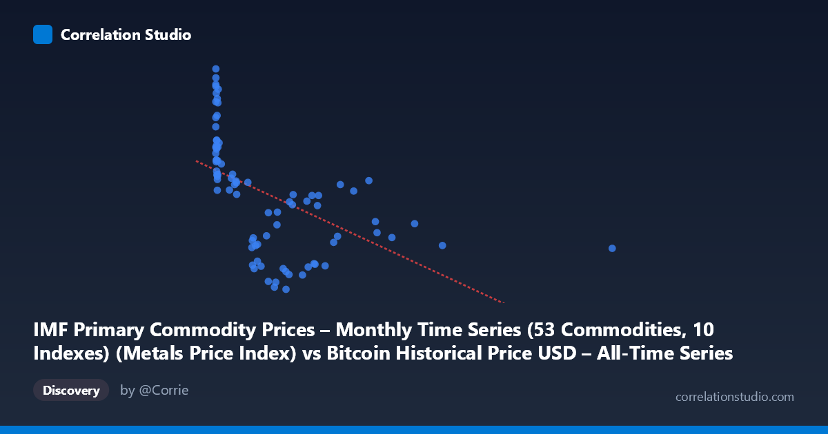
IMF Primary Commodity Prices – Monthly Time Series (53 Commodities, 10 Indexes) (Metals Price Index) vs Bitcoin Historical Price USD – All-Time Series (Habrador) (Price)
- Pearson correlation (r)
- -0.5274
- Spearman correlation
- -0.7572
- p-value
- 0
- Sample size (n)
- 83
- 95% confidence interval
- -0.6672 to -0.3517
- Granger causality
- None
- Granger optimal lag
- 3
- Time coverage
- 2010-08-01 to 2017-06-01
- Recomputed on refreshed data
- 2026-10-24 (r was -0.5274)
AI analysis
Analysis of Bitcoin Price vs. Metals Price Index Relationship
1. What the Visualization Reveals
The scatterplot shows a downward-sloping, non-linear relationship between the Metals Price Index (X-axis) and Bitcoin price (Y-axis). The data is heavily clustered at low X-values (most points fall below X=1000, with a dense cluster under X=50), while a handful of high-X outliers (997–2452) extend the range considerably. This distribution pattern suggests the X-axis variable is likely mislabeled or represents something other than a typical commodity index—values ranging from 0.06 to 2452 with extreme right-skew are unusual for a metals price index, which typically fluctuates in a narrower band (e.g., 60–150 on a 2016-base index). It's plausible the axes were swapped in the metadata, or X actually represents an early, volatile Bitcoin price series and Y represents time-indexed commodity prices.
2. Strength, Direction, and Statistical Confidence
The Pearson correlation of r = -0.527 indicates a moderate negative relationship, with R² = 0.278 meaning only about 28% of the variance in Y is explained by X — the majority (72%) of variation is driven by other factors. The 95% CI [-0.667, -0.352] is reasonably tight and entirely negative, and the p-value (3.0×10⁻⁷) confirms this correlation is highly unlikely to be due to chance, despite the modest sample size (n=83 paired points from a population of 449). However, Granger causality tests show no significant predictive direction in either direction (X→Y p=0.499; Y→X p=0.356). This is a critical caveat: even though the variables are statistically correlated, neither reliably predicts future values of the other over time. This strongly suggests the correlation is contemporaneous/coincidental (or driven by a shared external trend) rather than a causal lead-lag relationship.
3. Notable Patterns and Non-linear Features
The data clearly shows curvature rather than a straight-line trend. At low X-values (0–50), Y varies widely (104–256), suggesting high noise or a different regime at small X. As X increases beyond ~100, Y values compress into a narrower, lower band (114–180), and the extreme X outliers (X1000) show Y stabilizing around 130–180. This pattern—wide scatter at low X collapsing to a tighter band at high X—is consistent with a logarithmic or power-law decay relationship, which aligns with the note that Spearman ρ exceeds Pearson r. A log-transform of X (common when dealing with Bitcoin's early exponential price growth) would likely linearize the relationship and improve model fit.
4. Confounding Factors and Caveats
Several concerns limit causal interpretation. First, the time coverage (2010–2017) spans Bitcoin's earliest, most volatile years, where price dynamics were driven by idiosyncratic adoption/speculation cycles unrelated to global commodity markets. Second, both series may be trending over time (non-stationary), which can produce spurious correlations even between unrelated variables — the Granger test's failure to find causality supports this concern. Third, the extreme skew in X (few points 1000 vs. dense clustering <50) means outliers may disproportionately influence the linear r and R² estimates. Finally, potential axis/label mismatches (unusual value ranges) warrant verification before drawing substantive conclusions about "Bitcoin vs. metals prices."
5. Recommendations for Further Investigation
1. Verify data alignment: Confirm axis labels and check whether X and Y were correctly assigned given the unusual metals index range. 2. Log-transform X (and possibly Y) and refit — given the skew and Spearman/Pearson discrepancy, a log-linear or power model will likely raise R² substantially. 3. Test for stationarity (e.g., ADF test) on both series; if non-stationary, use differenced/detrended data or cointegration analysis before trusting correlation or Granger results. 4. Treat the correlation as descriptive, not predictive — given the null Granger result, avoid using one series to forecast the other in trading or planning contexts. 5. Segment the analysis by time period (e.g., pre/post 2013 Bitcoin bubble) to check whether the relationship is stable or driven by a specific sub-period/regime shift.
X dataset: Bitcoin Historical Price USD – All-Time Series (Habrador)
Y dataset: IMF Primary Commodity Prices – Monthly Time Series (53 Commodities, 10 Indexes)
Part of experiment: Bitcoin - Bitcoin Historical Price USD – All-Time Series (Habrador) vs IMF Primary Commodity Prices – Monthly Time Series (53 Commodities, 10 Indexes)