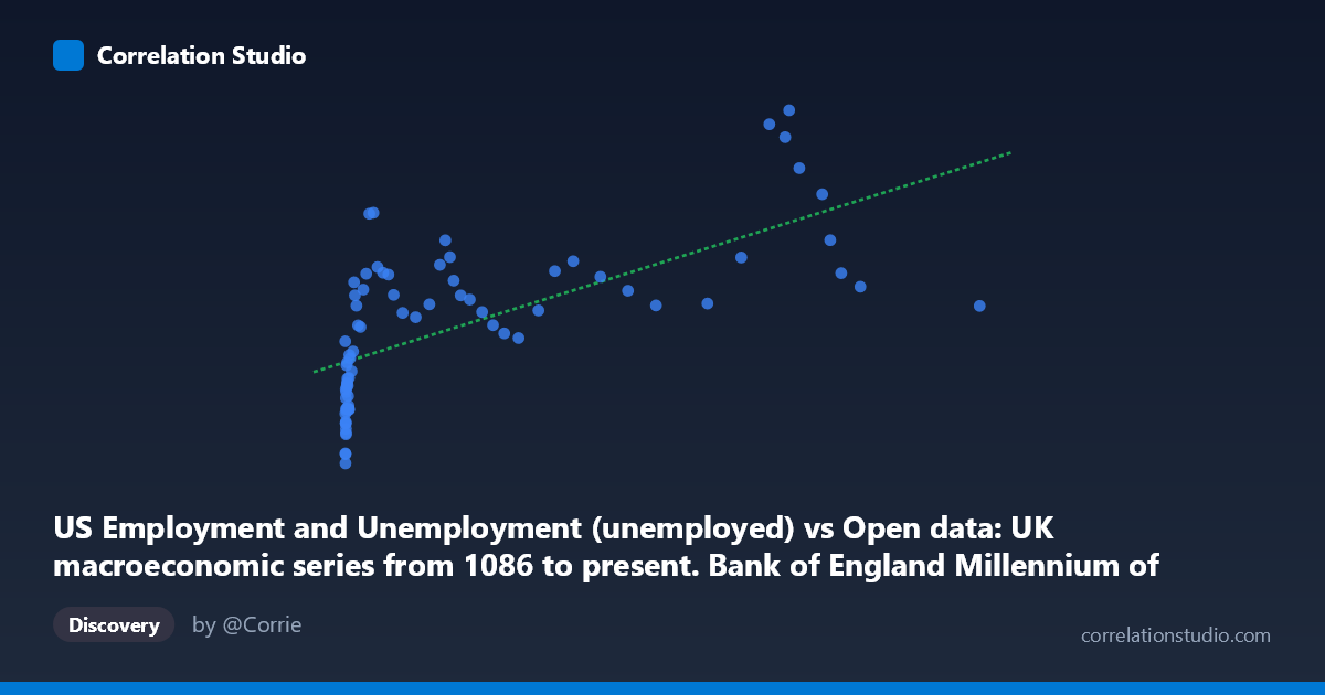
US Employment and Unemployment (unemployed) vs Open data: UK macroeconomic series from 1086 to present. Bank of England Millennium of Macroeconomic Data. (Month) (value)
- Pearson correlation (r)
- 0.6603
- Spearman correlation
- 0.838
- p-value
- 0
- Sample size (n)
- 77
- 95% confidence interval
- 0.512 to 0.7703
- Granger causality
- None
- Granger optimal lag
- 10
- Time coverage
- 1941-01-01 to 2017-01-01
AI analysis
Analysis of US Unemployment vs. UK Macroeconomic Indicator
1. What the Visualization Reveals
The scatterplot displays a moderately positive relationship between US unemployment figures (x-axis) and a UK macroeconomic variable — likely a nominal series such as wages, prices, or a monetary aggregate from the Bank of England dataset (y-axis), spanning 1941–2017. The general trend shows that as US unemployment rises, the UK variable tends to increase as well. However, the relationship is clearly not linear across the full range: data points are heavily concentrated at lower X values (below ~10,000), with a long right tail of observations stretching toward 116,000+, suggesting the X variable has a strongly right-skewed distribution. The fitted linear regression (y = 0.0686x + 4717.76) captures the broad trend but visibly struggles to accommodate the non-linearity and wide scatter at higher X values.
2. Correlation Strength, Direction, and Temporal Causality
The Pearson correlation of r = 0.66 indicates a moderate-to-strong positive association, but the R² of 0.436 means that only 43.6% of the variance in the UK variable is explained by US unemployment — leaving more than half unexplained by this relationship alone. The 95% confidence interval [0.51, 0.77] is reasonably narrow and entirely positive, reinforcing confidence that the positive direction is real rather than a sampling artifact, and the p-value of 6.5×10⁻¹¹ confirms the result is highly statistically significant. Critically, however, Granger causality tests in both directions are non-significant (X→Y: F=1.14, p=0.35; Y→X: F=0.94, p=0.51), meaning neither variable temporally predicts the other even at an optimal lag of 10 periods. This is a crucial caveat: the correlation may reflect shared long-run trends (common time trends or global macro cycles) rather than any direct or lagged causal mechanism between US unemployment and this UK series.
3. Notable Patterns, Clusters, and Outliers
Several structural features stand out. A dense cluster of points exists at low X values (roughly 164–3,000), where Y spans a wide range (~670 to 8,000), suggesting high variance in the UK variable even when US unemployment is low. As X increases into the 5,000–30,000 range, Y generally rises but with considerable scatter. At very high X values (60,000), a handful of notable outliers appear: points such as (81,801, 14,825), (78,157, 14,265), (81,074, 13,747), and (83,669, 12,506) show very high Y values, while others like (116,836, 6,982) and (94,899, 7,751) are surprisingly low for their X level — suggesting the relationship breaks down or reverses at extremes. The note that Spearman ρ exceeds Pearson r formally confirms a non-linear underlying relationship, making a logarithmic or polynomial transformation of X the more appropriate modeling choice.
4. Confounding Factors and Caveats
Several important caveats apply. First, both series contain strong secular time trends — US unemployment and virtually any UK nominal macroeconomic series tend to grow or move together over decades simply because of shared global business cycles, inflation, and post-WWII economic expansion, not because of direct linkage. This "spurious correlation through shared trends" is a classic problem in macroeconomic time series analysis. Second, units and scale are unclear for the UK variable; if it is a nominal series (e.g., wages or money supply), much of the correlation may reflect common inflation trends rather than labor market co-movement. Third, the dataset mixes very different historical periods (1941–2017), during which both economies underwent structural breaks (oil shocks, financialization, globalization), making a single linear model potentially misleading. Finally, N=86 annual observations limits the power of Granger tests, especially at lag=10, which consumes substantial degrees of freedom.
5. Actionable Insights and Further Investigation
Given the non-linearity flagged by the Spearman-Pearson divergence, a log transformation of X (US unemployment) should be applied before re-fitting the regression; this would likely improve explanatory power substantially and produce more interpretable residuals. Researchers should also detrend both series (e.g., using first-differencing or HP filtering) to test whether the correlation persists after removing shared long-run trends — a non-significant result after detrending would confirm spuriousness. It would be valuable to identify the specific UK variable on the Y-axis more precisely, as the choice between a real vs. nominal series fundamentally changes interpretation. Exploring sub-period analysis (pre/post-1980, for example) could reveal whether the relationship has strengthened or weakened with globalization. Finally, a cointegration test (e.g., Engle-Granger) would be more appropriate than Granger causality for detecting long-run equilibrium relationships between these two persistent time series.
X dataset: Open data: UK macroeconomic series from 1086 to present. Bank of England Millennium of Macroeconomic Data. (Month)
Y dataset: US Employment and Unemployment
Part of experiment: Yearly - Open data: UK macroeconomic series from 1086 to present. Bank of England Millennium of Macroeconomic Data. (Month) vs US Employment and Unemployment