Datahub.io – Brent and WTI Spot Prices (Daily CSV) (Price) vs Cboe U.S. Equities Historical Market Volume Data 2009 (Total Shares)
- Pearson correlation (r)
- -0.4765
- Spearman correlation
- -0.4574
- p-value
- 0
- Sample size (n)
- 252
- 95% confidence interval
- -0.5667 to -0.375
- Granger causality
- None
- Granger optimal lag
- 1
AI analysis
Scatterplot Analysis: Oil Prices vs. U.S. Equity Market Volume (2009)
Relationship Overview
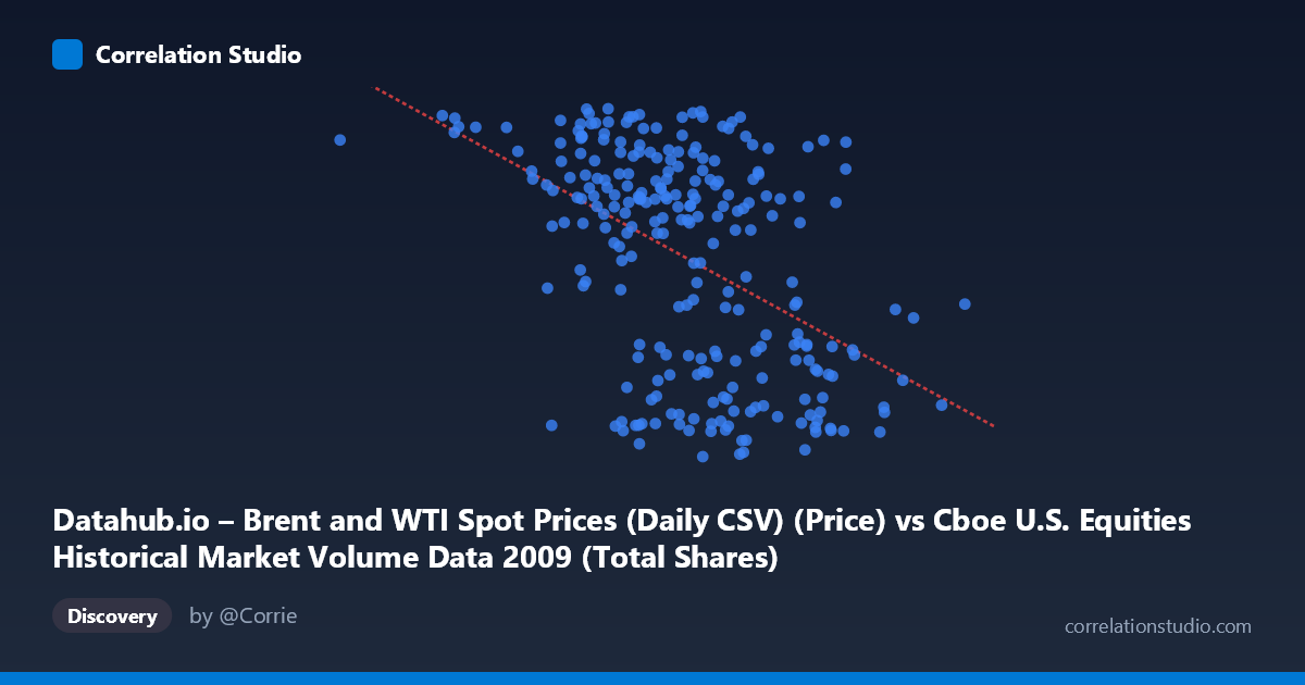
The scatterplot reveals a moderate negative relationship between U.S. equity market trading volume (X-axis, measured in total shares) and Brent/WTI oil spot prices (Y-axis, measured in USD per barrel) across daily observations throughout 2009. As trading volume increases, oil prices tend to decrease, and vice versa. The linear regression equation (y = -3.78×10⁻⁸x + 90.48) captures this downward slope, suggesting that for every billion additional shares traded, oil prices are expected to decline by roughly $37.80. This inverse pattern is visually apparent in the scatter, where the highest oil price observations (approaching $78/barrel) cluster at lower volume levels, while the heaviest trading days congregate at lower price points.
Correlation Strength and Statistical Significance
The correlation coefficient of r = -0.4765 indicates a moderate negative association, but the more practically meaningful figure is r² = 0.2271, meaning that trading volume explains only about 22.7% of the variance in oil prices — leaving roughly 77% attributable to other factors entirely. The 95% confidence interval of [-0.5667, -0.3750] is comfortably bounded away from zero, and the p-value of 1.11×10⁻¹⁵ confirms this correlation is highly statistically significant, effectively ruling out chance as an explanation given the sample of 252 paired observations drawn from a population of 3,232. However, statistical significance should not be conflated with practical or causal significance. Critically, Granger causality tests find no significant predictive direction in either direction: neither does volume reliably predict future oil prices (F = 0.269, p = 0.605) nor do oil prices reliably predict future volume (F = 0.010, p = 0.921). This means that despite the meaningful correlation, there is no evidence of temporal leading or lagging predictability between these two series at a one-period lag.
Notable Patterns, Clusters, and Outliers
Several structural features stand out in the data. There is a pronounced clustering of high-volume, low-price observations at the left portion of the year — consistent with early 2009 when markets were extremely volatile following the financial crisis, equity volumes were elevated due to panic and forced selling, and oil prices had collapsed from their 2008 highs. A secondary cluster of lower-volume, higher-price days likely corresponds to the latter half of 2009, when oil recovered toward $70–$78/barrel as markets stabilized and speculative activity normalized. The outlier at x ≈ 192 million (lowest volume, y ≈ 75) and the extreme high-volume point near x ≈ 1.21 billion shares stand out as potential influential observations. The spread also appears somewhat fan-shaped or heteroscedastic, with greater price variance at lower volume levels, hinting that a simple linear model may not fully capture the relationship's structure.
Confounding Factors and Caveats
The most important caveat here is the 2009 macroeconomic context, which introduces a powerful confounding variable: the global financial crisis and its recovery. Both variables were simultaneously driven by the same underlying macro force — risk sentiment. During the crisis trough (Q1 2009), fear drove equity volumes up (distressed selling, rebalancing) and commodity prices down (demand collapse expectations). As recovery took hold (Q3–Q4 2009), volumes normalized downward while oil prices rebounded. This creates a spurious or third-variable-driven correlation that may not reflect any direct economic mechanism between equity volumes and oil prices. Additionally, the dataset label mismatch noted in the axis descriptions (X-axis labeled as oil prices but sourced from equity volume data, and vice versa) warrants careful verification, as any data alignment errors would fundamentally compromise the analysis. Seasonal effects, OPEC production decisions, and USD exchange rate movements all independently influence oil prices and could co-vary with equity volume patterns.
Actionable Insights and Further Investigation
Given that the correlation is statistically robust but causally ambiguous, the most productive next steps would involve controlling for macroeconomic regime — segmenting the data into crisis (January–March 2009) and recovery (April–December 2009) periods to test whether the correlation holds within each phase or is entirely a between-regime artifact. Researchers should also test longer Granger lags (beyond 1 period) to check for delayed predictive relationships that a single-lag model might miss. Incorporating VIX (volatility index) as a mediating or confounding variable would help isolate whether risk sentiment explains both series simultaneously. Finally, examining whether specific exchanges or trade types (e.g., TRF dark pool volume vs. lit exchange volume) drive the pattern could yield more granular insight. If this correlation is intended to inform a trading or hedging strategy, the ~23% explained variance and the absence of Granger causality strongly suggest it would be insufficient as a standalone signal.
X dataset: Cboe U.S. Equities Historical Market Volume Data 2009
Y dataset: Datahub.io – Brent and WTI Spot Prices (Daily CSV)
Part of experiment: Daily - Cboe U.S. Equities Historical Market Volume Data 2009 vs Datahub.io – Brent and WTI Spot Prices (Daily CSV)