NOAA ISD Weather Station History (Lat/Lon Index) (SLP_ATTRIBUTES) vs Bitcoin Historical Price USD – All-Time Series (Habrador) (Price)
- Pearson correlation (r)
- -0.472
- Spearman correlation
- -0.3071
- p-value
- 0
- Sample size (n)
- 355
- 95% confidence interval
- -0.5491 to -0.3869
- Granger causality
- None
- Granger optimal lag
- 1
AI analysis
Scatterplot Analysis: Weather Station Index vs. Bitcoin Price
1. What the Visualization Reveals
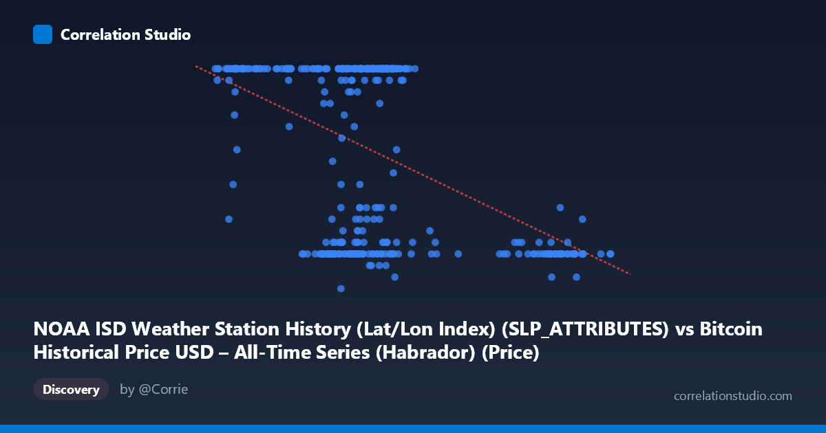
The scatterplot shows a moderate negative relationship between the two variables, with a clear downward-sloping trend as X increases. However, the data is not uniformly distributed along a line — there's a dense cluster of points where Y sits at or near the ceiling value of 24, spanning a wide range of X values (roughly 40,000–72,000), alongside a scattered lower band of points (Y between 7–12) occupying a similar X range. This bimodal clustering, rather than a smooth linear scatter, suggests the "negative correlation" is partly an artifact of two overlapping populations rather than a single continuous relationship.
2. Strength, Direction, and Statistical Interpretation
The correlation coefficient (r = -0.472) indicates a moderate negative relationship, with r² = 0.223 meaning only about 22% of the variance in Y is statistically explained by X — leaving nearly 78% unexplained by this linear model alone. The 95% CI [-0.549, -0.387] is reasonably tight and excludes zero, and the p-value of ~0 confirms the correlation is statistically significant and not due to random chance, given n=355. However, statistical significance here reflects sample size more than practical predictive strength — r² of 0.22 is a weak-to-moderate effect size in practical terms. Critically, the Granger causality tests show no significant predictive direction in either direction (X→Y: p=0.58; Y→X: p=0.27), meaning that despite the contemporaneous correlation, neither variable helps forecast the other's future values in a time-lagged sense. This strongly suggests the relationship is either coincidental, driven by a shared external factor, or purely structural/cross-sectional rather than causal or temporally dynamic.
3. Notable Patterns and Outliers
The most striking feature is the ceiling effect at Y=24 — a large number of points cluster exactly at this value across diverse X values, suggesting Y may be capped, clipped, or aggregated (e.g., a maximum daily value, or an artifact of data joining/resampling). Separately, there's a distinct low-Y cluster (Y ≈ 7–12) concentrated in two X sub-ranges: one around 58,000–72,000 and another at higher X values (89,000–101,000+), where nearly all points have low Y. This suggests at least two distinct regimes or subpopulations in the data rather than one continuous trend, which would violate assumptions of simple linear correlation and inflate or distort the r value.
4. Confounding Factors and Caveats
The variable labeling here is unusual and likely mismatched: the X-axis is described as a NOAA weather station lat/lon index while the Y-axis is labeled as Bitcoin price, but the dataset descriptions suggest the reverse mapping (X = Bitcoin price history, Y = weather station attributes). This strongly implies a column-mapping error in the data pipeline, and any interpretation should be treated cautiously until the axis assignments are verified. Additionally, pairing daily weather station identifiers/attributes with Bitcoin price data has no plausible causal mechanism — this is very likely a spurious correlation arising from coincidental time alignment (both span 2024-01-01 to 2024-12-31) rather than genuine covariation. The ceiling clustering at Y=24 also hints at data quality issues (capping, encoding of categorical values as numeric, or merge artifacts) that could mechanically produce correlation without meaning.
5. Recommendations for Further Investigation
Before drawing any substantive conclusions, verify the actual data source and column mapping — the mismatch between axis labels and dataset descriptions needs correction. Investigate the Y=24 ceiling cluster specifically: determine whether this represents a true maximum, a default/missing-value placeholder, or a categorical code (e.g., "24" could represent hours, a station attribute code, or a capped scale) that shouldn't be treated as continuous. Given the lack of Granger causality in either direction, this pairing should not be used for forecasting purposes. If a genuine relationship is suspected, consider re-running the analysis after removing or separately modeling the two apparent clusters, and formally test for a plausible confounding variable (e.g., time-of-year, station region, or a third joined dataset key) that might explain both series' patterns independently.
X dataset: Bitcoin Historical Price USD – All-Time Series (Habrador)
Y dataset: NOAA ISD Weather Station History (Lat/Lon Index)
Part of experiment: Bitcoin - Bitcoin Historical Price USD – All-Time Series (Habrador) vs NOAA ISD Weather Station History (Lat/Lon Index)