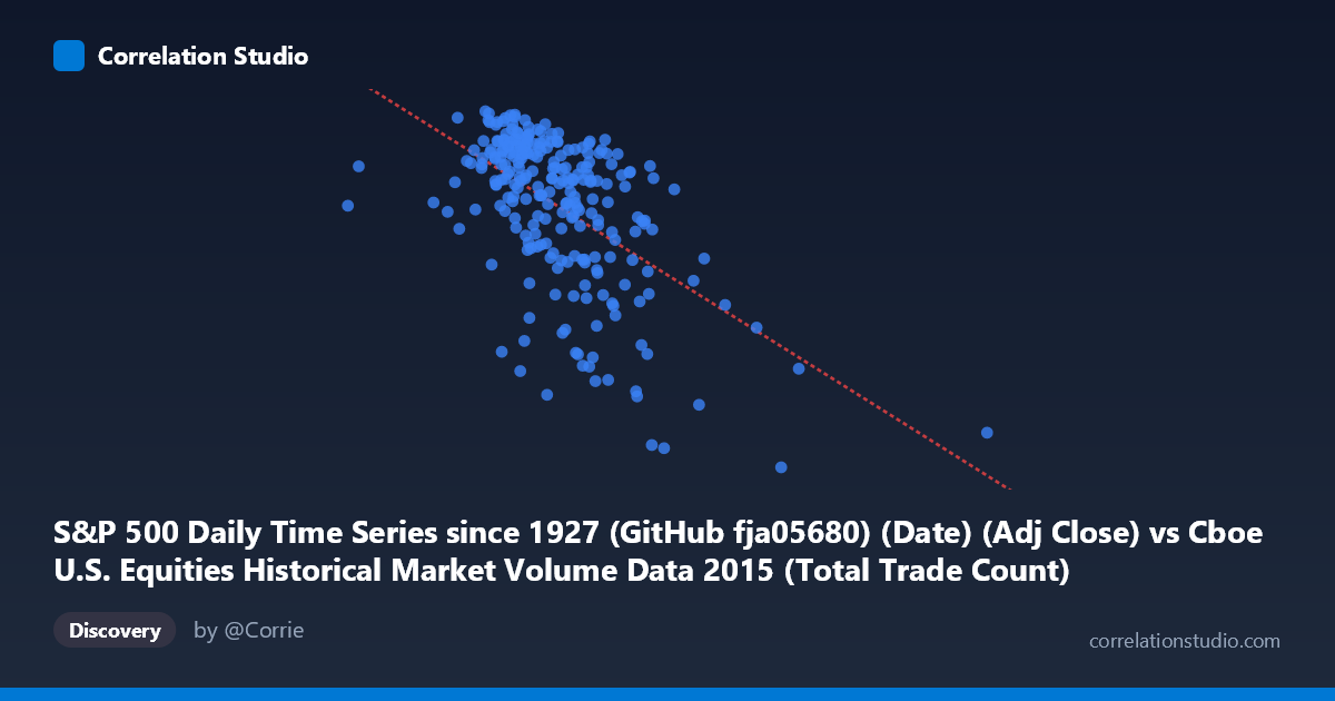
S&P 500 Daily Time Series since 1927 (GitHub fja05680) (Date) (Adj Close) vs Cboe U.S. Equities Historical Market Volume Data 2015 (Total Trade Count)

Pearson correlation (r): -0.5523
Spearman correlation: -0.5192
p-value: 0
Sample size (n): 252
95% confidence interval: -0.6327 to -0.4601
Granger causality: None
Granger optimal lag: 1

AI analysis

S&P 500 Price vs. U.S. Equity Trade Count (2015)

Relationship Overview The scatterplot reveals a moderate negative relationship between the S&P 500 adjusted closing price (X) and the total U.S. equity trade count (Y) across 2015 trading days. As the S&P 500 price level rises, the number of daily trades tends to decline, and conversely, periods of lower index prices correspond to higher trading activity. The linear regression equation (y = −6.515×10⁻⁵x + 2223.03) quantifies this inverse slope, suggesting that for every ~15,000-point increase in the S&P 500, trade count drops by roughly one unit on the Y scale — though the practical interpretation depends heavily on the units of the trade count variable.

Correlation Strength and Statistical Reliability The Pearson correlation of r = −0.5523 indicates a moderate negative association, but the explanatory power is more sobering: r² = 0.305 means only ~30.5% of the variance in trade count is explained by S&P 500 price level, leaving nearly 70% attributable to other factors. The 95% confidence interval of [−0.633, −0.460] is reasonably tight and sits entirely in negative territory, confirming directional reliability. The p-value of effectively 0 (with N = 3,302) confirms this is not a chance finding. However, Granger causality tests show no significant temporal predictive relationship in either direction (X→Y: F = 0.29, p = 0.59; Y→X: F = 0.41, p = 0.52), meaning that yesterday's S&P 500 price does not reliably predict today's trade count, and vice versa. This is a critical caveat: the correlation is contemporaneous and structural, not predictive in a causal time-series sense.

Notable Patterns and Outliers Several features stand out in the data. The bulk of observations cluster in the X range of ~1,900,000–2,700,000 with Y values between roughly 2,025 and 2,130, forming a relatively dense core. However, there is a visible lower-right tail where higher X values (e.g., 3,907,922 and 4,083,023) correspond to notably low Y values (~1,868–1,971), including what appears to be a clear outlier near (4,083,023, 1,867.61) — the lowest trade count in the dataset. There are also low-X outliers (e.g., 997,371) that appear isolated from the main cluster. The spread in Y widens at intermediate X values, suggesting heteroscedasticity — the relationship may not be uniformly linear across the full price range, and a non-linear or piecewise model might better describe the tails.

Confounding Factors and Caveats Several important confounders likely drive this correlation. Market volatility is a well-known driver of trading volume and trade count — high-volatility periods (often associated with market declines) naturally generate more transactions as traders react to price swings. This means the negative correlation may be largely mediated by volatility rather than price level per se. Additionally, seasonality plays a role in 2015 equity markets (e.g., the August 2015 correction inflated both volatility and trade counts while depressing prices). The dataset covers only a single calendar year, limiting generalizability — 2015 included a notable late-summer selloff that could be disproportionately influencing the correlation. The unit of trade count (likely millions or thousands of trades) and its aggregation across all U.S. exchanges including TRFs also introduces structural variation unrelated to S&P 500 dynamics.

Actionable Insights and Further Investigation Given these findings, several investigative steps would sharpen understanding. First, controlling for realized volatility (e.g., VIX) as a covariate would help isolate whether price level itself drives trade count or whether volatility is the true underlying driver. Second, segmenting the data by market regime (trending vs. corrective periods in 2015) could reveal whether the relationship holds uniformly or is concentrated in specific episodes like the August selloff. Third, testing with longer time horizons across multiple years would establish whether this −0.55 correlation is stable or an artifact of 2015's particular market structure. Finally, since Granger causality was insignificant at lag 1, exploring longer lag structures or using a VAR model with additional variables (volatility, bid-ask spreads, macroeconomic news flow) could uncover richer predictive dynamics between market prices and market microstructure activity.

X dataset: Cboe U.S. Equities Historical Market Volume Data 2015

Y dataset: S&P 500 Daily Time Series since 1927 (GitHub fja05680) (Date)

Part of experiment: Daily - Cboe U.S. Equities Historical Market Volume Data 2015 vs S&P 500 Daily Time Series since 1927 (GitHub fja05680) (Date)