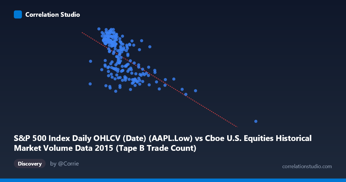
S&P 500 Index Daily OHLCV (Date) (AAPL.Low) vs Cboe U.S. Equities Historical Market Volume Data 2015 (Tape B Trade Count)
- Pearson correlation (r)
- -0.6072
- Spearman correlation
- -0.6048
- p-value
- 0
- Sample size (n)
- 222
- 95% confidence interval
- -0.6841 to -0.5168
- Granger causality
- None
- Granger optimal lag
- 1
AI analysis
Scatterplot Analysis: AAPL Low Price vs. Cboe Tape B Trade Count (2015)
1. Relationship Overview The scatterplot reveals a negative relationship between Apple's daily low price (X-axis) and the Cboe U.S. Equities Tape B trade count (Y-axis) over the period February–December 2015. As AAPL's low price increases, Tape B trade counts tend to decrease, and vice versa. The linear regression equation (y = -4.87e-05x + 134.06) confirms this inverse slope, suggesting that for every unit increase in AAPL's low price, Tape B trade counts decline by a small but consistent margin. The bulk of data points cluster in the lower-left region of the chart, with a visible downward trend, though with considerable scatter around the regression line.
2. Correlation Strength, Direction, and Causality The Pearson correlation of r = -0.607 indicates a moderate-to-strong negative association, and the R² of 0.369 means that approximately 36.9% of the variance in Tape B trade counts is explained by AAPL's low price — a meaningful but far from complete explanatory relationship. The 95% confidence interval of [-0.684, -0.517] is entirely negative and relatively narrow given n = 222, reinforcing confidence that the true population correlation is genuinely negative and non-trivial. The p-value of ~0 confirms this relationship is highly statistically significant and extremely unlikely to be a chance finding. However, Granger causality tests reveal no significant temporal predictive direction in either direction (X→Y: F = 0.888, p = 0.347; Y→X: F = 0.185, p = 0.667), meaning that neither variable reliably predicts future values of the other at a one-period lag. This critically distinguishes co-movement from causal or predictive influence — the correlation is real, but neither series temporally leads the other in a statistically meaningful way.
3. Notable Patterns, Clusters, and Outliers The data exhibits a tight cluster of observations where AAPL low prices fall between roughly $200,000–$400,000 (in the dataset's units) and Tape B trade counts between approximately 108–131, suggesting typical market conditions dominate most of the sample. There are two prominent outliers worth noting: one point at approximately (1,014,194, 92.00) represents an extreme X value — nearly three times the next-highest observation — paired with the lowest observed Y value, likely corresponding to a market stress or anomalous volume event. A second outlier near (640,679, 103.50) similarly sits far from the main cluster. These high-leverage points almost certainly exert disproportionate influence on the regression slope and correlation coefficient, potentially inflating the magnitude of the negative correlation.
4. Confounding Factors and Caveats Several important caveats apply. First, the dataset description appears to mix metadata: AAPL Low prices are labeled as originating from a Cboe market volume dataset, and Tape B trade counts from an S&P 500 OHLCV dataset, suggesting possible data pipeline or column-mapping issues that warrant verification before drawing conclusions. Second, this is a cross-market, cross-asset correlation — AAPL's price behavior and Tape B (NYSE American/regional exchange) trade counts are influenced by distinct but partly overlapping macroeconomic forces (e.g., broad market volatility, institutional rebalancing, sector rotation), making common-cause confounding highly plausible. The August 2015 market correction, which would affect both AAPL prices and overall trade volumes simultaneously, is a strong candidate confound. Third, with ~63% of variance unexplained, many other drivers remain unaccounted for.
5. Actionable Insights and Further Investigation Given the absence of Granger causality, this correlation should not be used for trading signals or short-term forecasting in its current form. However, the moderate correlation and high significance suggest a genuine structural link worth exploring. Recommended next steps include: (a) verifying column-to-dataset assignments to rule out labeling errors; (b) removing or analyzing the two extreme outliers separately to assess their influence on the regression; (c) introducing volatility measures (e.g., VIX) and broader market volume as control variables to test whether the AAPL-Tape B relationship persists after accounting for market-wide conditions; (d) testing non-linear models (e.g., logarithmic or piecewise regression), since the outlier structure suggests the relationship may not be uniformly linear across the full price range; and (e) extending the Granger analysis to longer lags (2–5 periods) to rule out delayed predictive effects.
X dataset: Cboe U.S. Equities Historical Market Volume Data 2015
Y dataset: S&P 500 Index Daily OHLCV (Date)
Part of experiment: Daily - Cboe U.S. Equities Historical Market Volume Data 2015 vs S&P 500 Index Daily OHLCV (Date)