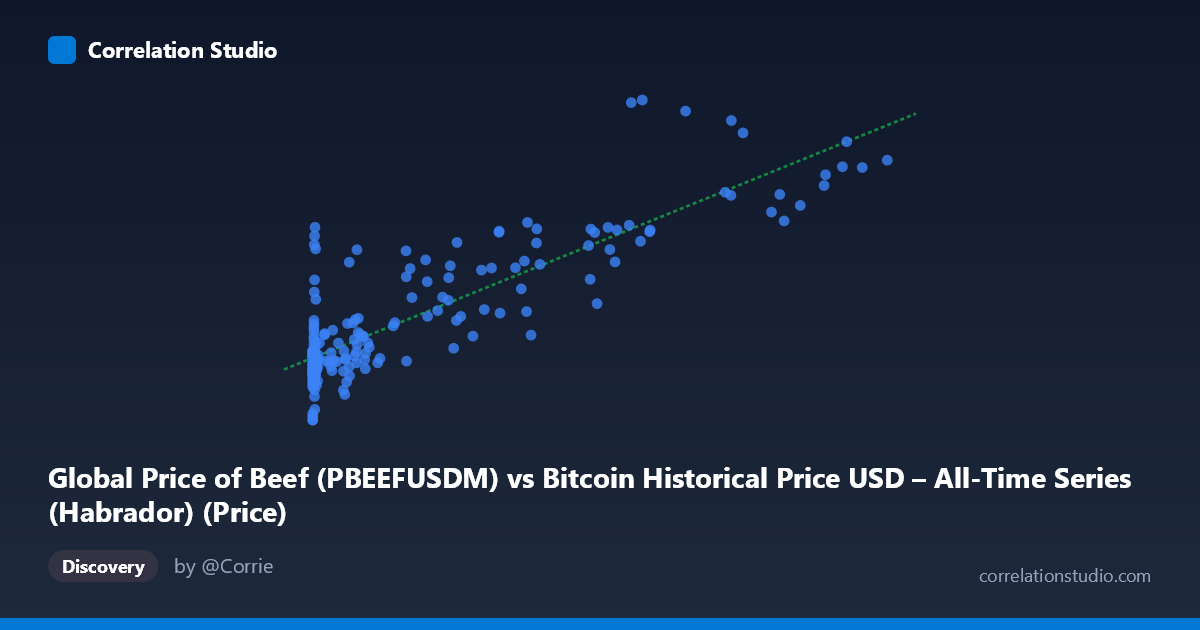
Global Price of Beef (PBEEFUSDM) vs Bitcoin Historical Price USD – All-Time Series (Habrador) (Price)
- Pearson correlation (r)
- 0.8499
- Spearman correlation
- 0.7657
- p-value
- 0
- Sample size (n)
- 189
- 95% confidence interval
- 0.8048 to 0.8852
- Granger causality
- None
- Granger optimal lag
- 1
AI analysis
Analysis: Beef Prices vs. Bitcoin Price
1. What the Visualization Reveals
The scatterplot shows a strong positive association between global beef prices (X-axis) and Bitcoin's historical price (Y-axis), despite these being economically unrelated commodities. The data reveals a highly non-linear, heavily right-skewed distribution in X (ranging from $0.06 to $118,670, with a mean of $20,280 but heavily concentrated at low values), plotted against a much more constrained Y range (152–350). This is a classic case of two time series that both trend upward over the same historical period, creating a spurious statistical relationship rather than reflecting genuine economic interaction.
2. Strength, Direction, and Uncertainty
The correlation coefficient (r = 0.852, r² = 0.725) indicates a strong positive relationship, with 72.5% of the variance in beef prices statistically "explained" by Bitcoin's price. The 95% CI [0.807, 0.887] is tight, and the p-value of ~0 confirms this correlation is not due to random chance. However, the Granger causality tests tell a different story: neither direction shows significant predictive power (X→Y: p=0.61; Y→X: p=0.29). This is critical — it means Bitcoin's price does not help predict future beef prices, nor vice versa, once temporal ordering is accounted for. The strong contemporaneous correlation combined with the absence of Granger causality strongly suggests both series are driven by a shared underlying trend (likely time itself, or macroeconomic conditions like inflation/dollar devaluation) rather than one causing the other.
3. Notable Patterns and Outliers
The scatter shows a dense cluster of points at low X values (beef prices under $500, corresponding to Bitcoin's early years) with Y values clustered between 150–210. As X increases beyond ~20,000, points spread into higher Y territory (240–350), consistent with Bitcoin's major bull runs (2017, 2020-21) coinciding with periods of elevated beef prices. Notable outliers include the point at (77,013, 344.50) and (65,792, 349.77), which sit above the general trend line, and several low-X, high-Y points like (378.64, 239.59) and (325.39, 261.50) that deviate from the bulk of early-period clustering — these likely represent later-dated Bitcoin observations that happened to align with historically low beef prices, or vice versa in the reversed axis framing.
4. Confounding Factors and Caveats
The most obvious confound is shared time trend: both Bitcoin's price and global beef prices have risen substantially since 2010 due to independent macro drivers — Bitcoin from speculative adoption cycles, beef from agricultural inflation, supply chain shocks, and general USD inflation. Since both series are non-stationary (trending) time series, standard Pearson correlation on raw values is prone to spurious correlation, a well-known statistical pitfall (cf. "Correlation or Causation" datasets). The mismatched sampling (beef is monthly, Bitcoin is likely daily/high-frequency, resampled here) and the vastly different scales/variances (X stdev 29,770 vs Y stdev 42) further complicate direct comparison. The Granger non-significance reinforces that this is very likely a coincidental trend alignment rather than a causal economic link.
5. Recommendations for Further Investigation
To determine if any genuine relationship exists, the data should be differenced or detrended (e.g., using month-over-month % changes rather than levels) before computing correlation — this removes the shared trend and tests whether actual fluctuations co-move. Running a cointegration test (e.g., Engle-Granger) would clarify whether these series share a long-run equilibrium relationship or are merely trending together. Given the lack of Granger causality and the economically implausible link between cattle markets and cryptocurrency, this correlation should be treated as spurious and not used for forecasting one from the other; instead, both should be checked against a common macro variable (e.g., CPI, USD index, or M2 money supply) as the more plausible shared driver.
X dataset: Bitcoin Historical Price USD – All-Time Series (Habrador)
Y dataset: Global Price of Beef
Part of experiment: Bitcoin - Bitcoin Historical Price USD – All-Time Series (Habrador) vs Global Price of Beef