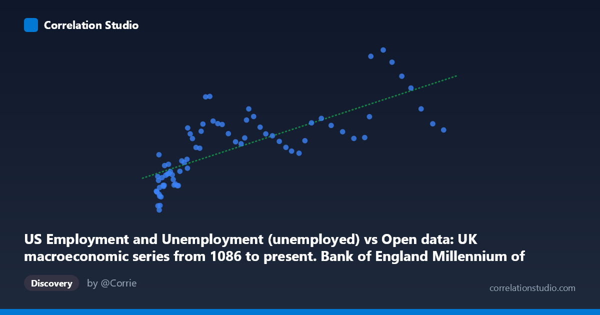
US Employment and Unemployment (unemployed) vs Open data: UK macroeconomic series from 1086 to present. Bank of England Millennium of Macroeconomic Data. (Year) (value)
- Pearson correlation (r)
- 0.7522
- Spearman correlation
- 0.8501
- p-value
- 0
- Sample size (n)
- 76
- 95% confidence interval
- 0.6343 to 0.8359
- Granger causality
- None
- Granger optimal lag
- 10
- Time coverage
- 1941-01-01 to 2016-01-01
AI analysis
Analysis: US Unemployment Numbers vs. UK Macroeconomic Values
1. Nature of the Relationship
The scatterplot reveals a moderately strong positive relationship between US unemployment figures (x-axis, ranging from ~33,000 to ~469,000) and UK macroeconomic values (y-axis, ranging from 670 to 14,825). The linear regression equation y = 0.019x + 3,250.68 indicates that for every additional 100,000 unemployed Americans, the UK measure increases by roughly 1,900 units. While the upward trend is discernible, the scatter around the regression line is substantial, suggesting considerable unexplained variation and hinting at a more complex underlying relationship than a simple linear model can capture.
2. Correlation Strength and Statistical Significance
The Pearson correlation of r = 0.752 reflects a moderately strong positive association, and with r² = 0.566, approximately 56.6% of the variance in the UK measure is statistically explained by US unemployment levels. The remaining 43.4% is attributable to other factors entirely. The 95% confidence interval [0.634, 0.836] is relatively tight and sits comfortably above zero, and the p-value of 4.9×10⁻¹⁵ renders this result overwhelmingly statistically significant — effectively ruling out chance as an explanation. However, despite this strong statistical signal, the Granger causality results are notably null: neither direction (X→Y: F=0.672, p=0.744; Y→X: F=0.233, p=0.991) achieves significance at any conventional threshold. This is a critical caveat — the correlation, however strong, carries no demonstrable temporal predictive power in either direction, suggesting the relationship is driven by shared underlying trends rather than one variable leading the other.
3. Notable Patterns, Clusters, and Outliers
Several structural features are visible in the data. A dense lower-left cluster exists at low US unemployment values (~33,000–100,000) paired with UK values mostly below 8,000, likely representing mid-20th century observations when both economies operated at historically lower scales. At higher unemployment values, the data fans out considerably — variance in the UK measure increases noticeably (heteroscedasticity), which undermines the assumptions of ordinary linear regression. Several notable outliers demand attention: the point at approximately (377,000, 14,825) sits well above the regression line, as does (390,530, 13,747), while (468,775, 7,751) sits substantially below what the model would predict for that unemployment level — suggesting the relationship breaks down at extremes. The point (37,673, 670) represents a historically low UK value that is also anomalously low for its x-position.
4. Confounding Factors and Interpretive Caveats
The most fundamental caveat here is that this correlation almost certainly reflects shared temporal trends rather than any genuine causal or structural economic link between US unemployment and a UK macroeconomic variable. Both series span 1941–2016, a period encompassing massive secular growth, post-war recoveries, recessions, and globalization — all of which would drive both variables upward over time simultaneously. This is a classic spurious correlation driven by common time trends. The Granger causality null result reinforces this interpretation. Additionally, the UK y-axis variable is described only generically, making substantive economic interpretation difficult — if it is a nominal series (e.g., nominal GDP, money supply), inflation alone could explain much of the apparent relationship. The mismatch in data provenance (US BLS employment data vs. Bank of England millennium series) and differing methodologies across decades add further noise.
5. Actionable Insights and Further Investigation
Before drawing any policy or economic conclusions, detrending both series (e.g., first-differencing or HP filtering) is essential to isolate cyclical co-movement from shared secular trends. Researchers should also clarify what the UK y-axis variable specifically represents, as the analysis is materially different depending on whether it measures nominal output, wages, or monetary aggregates. Applying cointegration tests (e.g., Engle-Granger) would determine whether the long-run relationship is economically meaningful or purely spurious. Given the visible heteroscedasticity, a log-log or semi-log transformation may produce a more stable and interpretable model. Finally, introducing control variables — global trade volumes, oil prices, or common business cycle indicators — would help isolate whether any residual US–UK relationship persists after removing shared global factors.
X dataset: Open data: UK macroeconomic series from 1086 to present. Bank of England Millennium of Macroeconomic Data. (Year)
Y dataset: US Employment and Unemployment
Part of experiment: Yearly - Open data: UK macroeconomic series from 1086 to present. Bank of England Millennium of Macroeconomic Data. (Year) vs US Employment and Unemployment