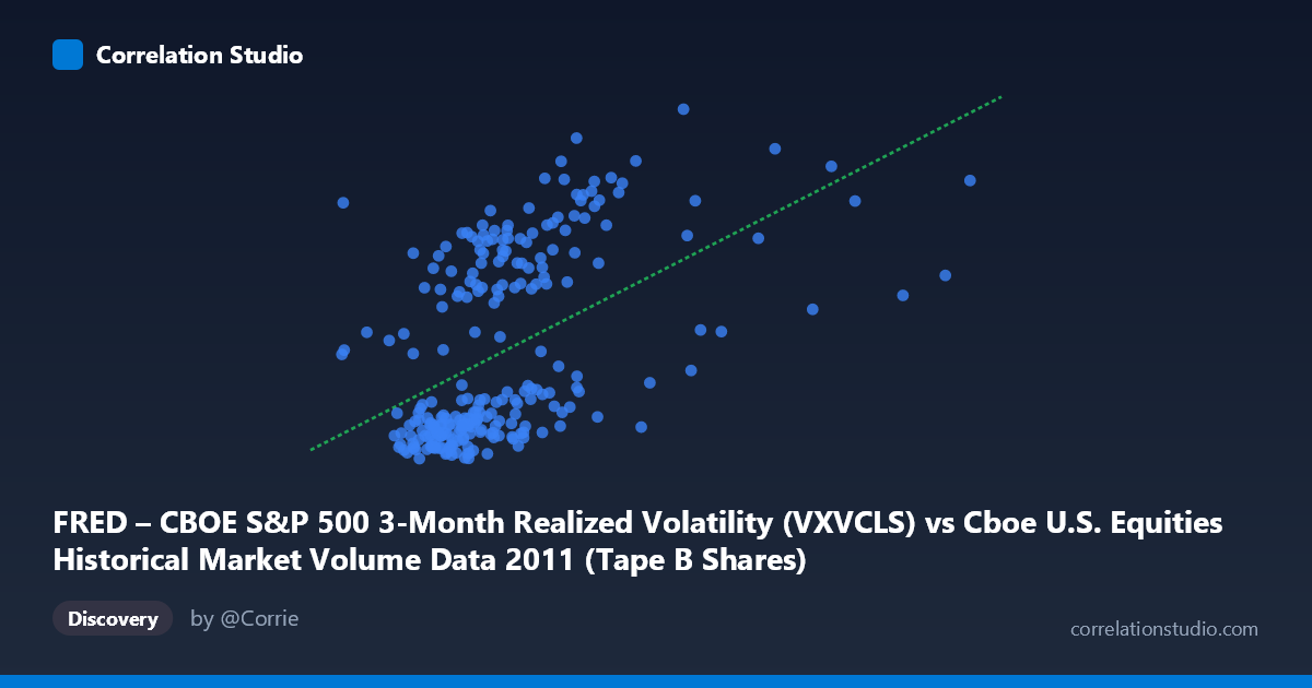
FRED – CBOE S&P 500 3-Month Realized Volatility (VXVCLS) vs Cboe U.S. Equities Historical Market Volume Data 2011 (Tape B Shares)
- Pearson correlation (r)
- 0.5039
- Spearman correlation
- 0.5843
- p-value
- 0
- Sample size (n)
- 252
- 95% confidence interval
- 0.4056 to 0.5907
- Granger causality
- None
- Granger optimal lag
- 1
AI analysis
Analysis: CBOE S&P 500 3-Month Realized Volatility vs. Tape B Shares Volume (2011)
Relationship Overview The scatterplot reveals a positive relationship between CBOE S&P 500 3-Month Realized Volatility (VXVCLS) and Tape B share trading volume across 2011. As realized volatility rises, Tape B share volume tends to increase as well — a relationship that aligns intuitively with market microstructure theory, where heightened uncertainty typically drives greater trading activity. However, the relationship is far from clean: considerable scatter around the regression line (y = 1.06×10⁻⁷x + 14.95) suggests that volatility is only one of several forces driving volume on these exchanges.
Correlation Strength and Statistical Framing The Pearson correlation of r = 0.504 indicates a moderate positive association, but the more informative metric is r² = 0.254 — meaning realized volatility explains only about 25.4% of the variance in Tape B share volume. Roughly three-quarters of volume variation is driven by factors outside this model. The 95% confidence interval of [0.406, 0.591] is meaningfully above zero and relatively tight given n = 252, and the p-value of effectively 0 confirms this association is not a statistical artifact. That said, statistical significance should not be conflated with practical magnitude — a quarter of variance explained leaves substantial unexplained noise. Critically, the Granger causality tests are non-significant in both directions (X→Y: F = 0.008, p = 0.929; Y→X: F = 0.136, p = 0.713), meaning that neither variable reliably predicts the other's future values at a one-period lag. The correlation is contemporaneous rather than predictive, limiting its utility for forecasting or causal inference.
Notable Patterns and Outliers The scatterplot exhibits several distinctive structural features. There appears to be a lower-bound floor in Tape B volume around the 17–20 range regardless of volatility level, suggesting a baseline trading activity that persists even in calm markets. At higher volatility readings (roughly above 30), volume values become more dispersed and extreme, creating a fan-shaped or heteroscedastic spread — variance in volume increases with volatility. Several high-leverage outliers are visible in the upper-right quadrant (e.g., points near X = 189M, Y = 33.8 and X = 176M, Y = 26.9), representing episodes where both volatility and volume spiked simultaneously, likely corresponding to specific market stress events in 2011 such as the U.S. debt ceiling crisis or European sovereign debt turbulence. A cluster of points with moderate-to-high Y values but relatively low X values also hints at non-linear dynamics.
Confounding Factors and Caveats Several important caveats apply. First, Tape B specifically covers NYSE American and regional exchange listings — a subset of total market volume — so findings may not generalize to broader market activity. Second, the axis labels appear potentially swapped in the dataset metadata (the X-axis is labeled as VXVCLS but draws from the volume dataset, and vice versa), which warrants verification before drawing firm conclusions. Third, 2011 was an unusually volatile year with multiple discrete shock events, meaning this sample may not represent typical volatility-volume dynamics. Fourth, the relationship may be driven by common external shocks (macro news, Fed announcements) that simultaneously spike both variables, producing correlation without direct causation — consistent with the failed Granger tests. Finally, the linear regression model may be misspecified; the fan-shaped scatter suggests a log-linear or power-law specification might better capture the true relationship.
Actionable Insights and Further Investigation Given the moderate but noisy correlation and absent Granger causality, practitioners should avoid using VXVCLS alone as a volume predictor in trading models. However, the association does support using volatility regimes as a conditioning variable — volume models could be stratified by low/medium/high volatility environments rather than using a single linear fit. Further investigation should include: (1) testing log-transformed variables to address heteroscedasticity and potential power-law dynamics; (2) expanding the time window beyond 2011 to assess whether the relationship is stable across different market regimes; (3) incorporating additional predictors such as VIX term structure, market breadth, or macroeconomic surprise indices to build a more complete volume model; and (4) examining whether the relationship strengthens at weekly or monthly aggregations, where noise averages out and structural relationships may emerge more clearly.
X dataset: Cboe U.S. Equities Historical Market Volume Data 2011
Y dataset: FRED – CBOE S&P 500 3-Month Realized Volatility
Part of experiment: Daily - Cboe U.S. Equities Historical Market Volume Data 2011 vs FRED – CBOE S&P 500 3-Month Realized Volatility