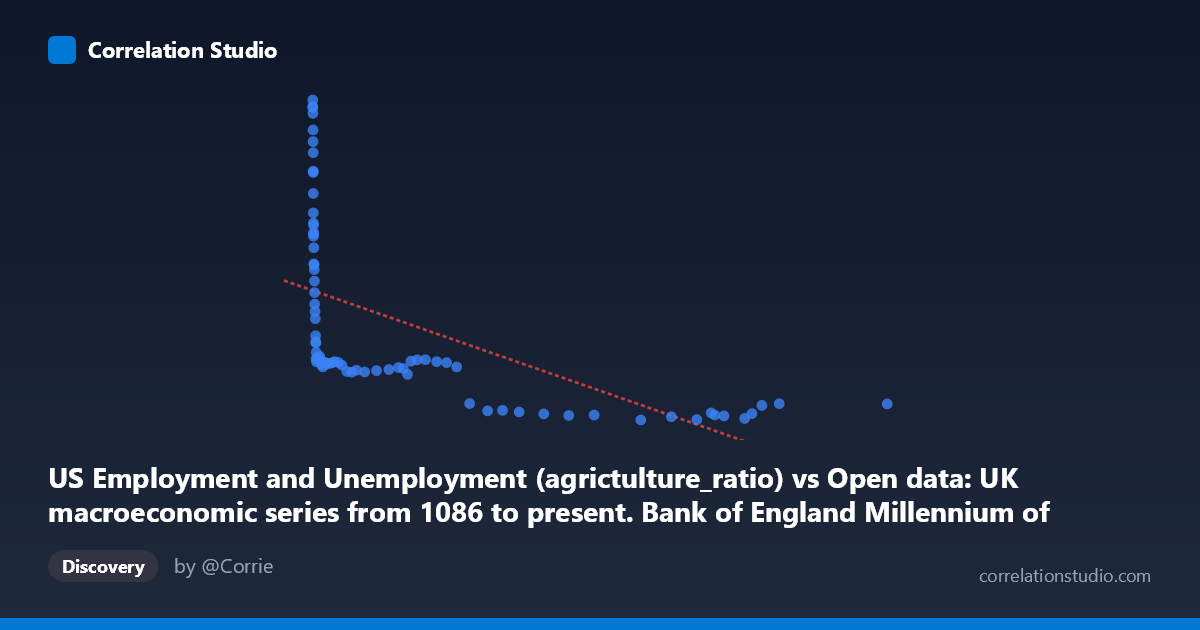
US Employment and Unemployment (agrictulture_ratio) vs Open data: UK macroeconomic series from 1086 to present. Bank of England Millennium of Macroeconomic Data. (Month) (value)
- Pearson correlation (r)
- -0.5775
- Spearman correlation
- -0.95
- p-value
- 0
- Sample size (n)
- 77
- 95% confidence interval
- -0.7097 to -0.4061
- Granger causality
- None
- Granger optimal lag
- 10
AI analysis
Analysis: UK Agriculture Ratio vs. US Employment Metric
1. Overall Relationship Pattern
The scatterplot reveals a negative, non-linear relationship between the UK agriculture employment ratio and the US employment/unemployment metric. At low X values (roughly below 2,000), Y values span a wide range from approximately 3,300 to 9,250, with many high Y values clustered in this region. As X increases beyond ~5,000, Y values compress dramatically into a narrow band between roughly 2,100 and 3,500. This pattern is characteristic of a logarithmic or power-law decay rather than a true linear relationship, meaning the linear regression equation (y = -0.038x + 4,996) likely understates the strength of the relationship at low X values while overstating it at high X values.
2. Correlation Strength and Statistical Significance
The Pearson r of -0.578 indicates a moderate negative correlation, but the R² of 0.334 tells us that only about 33.4% of the variance in Y is explained by X — meaning roughly two-thirds of the variation remains unexplained by this linear model alone. The 95% confidence interval of [-0.710, -0.406] is meaningfully wide, reflecting real uncertainty in the true population correlation, though it does not cross zero. The p-value of 3.83×10⁻⁸ confirms this is highly statistically significant and extremely unlikely to be a chance finding. Crucially, however, Granger causality tests in both directions are non-significant (X→Y: p=0.157; Y→X: p=0.270), meaning neither variable demonstrably predicts the other temporally at the optimal 10-period lag. This is an important caveat: the two series move together historically, but neither leads the other in a predictive sense.
3. Notable Patterns, Clusters, and Outliers
Several structural features stand out:
- Low-X cluster (X < 1,000): A dense cluster of points with highly variable Y values (ranging ~3,300–9,250), including what appear to be earlier historical observations when the UK agriculture ratio was small and US employment conditions were more varied. Points like (164, 9100), (176, 9250), and (210, 8950) suggest extreme Y values when X is near its minimum. - High-X plateau (X 40,000): A relatively tight cluster of points where Y is compressed between ~2,100 and 2,500, suggesting a floor effect — the US metric appears to reach a lower bound regardless of how large X becomes. - Transition zone (X = 1,000–10,000): Y values drop steeply and variability narrows, consistent with a logarithmic curve. - The Spearman ρ exceeding Pearson r explicitly flags a non-linear relationship, reinforcing that a logarithmic or power regression would fit the data substantially better.
4. Confounding Factors and Interpretive Caveats
Several important caveats apply here:
- Spurious cross-national correlation: These datasets come from fundamentally different national economies (UK macroeconomic data vs. US employment data), so any correlation almost certainly reflects shared temporal trends (e.g., both series evolving over the 1941–2017 period) rather than a direct economic mechanism. The agricultural ratio decline in the UK mirrors global structural economic shifts, as does long-run US employment evolution. - Temporal confounding: Both series are likely co-driven by long-run industrialization, globalization, and post-WWII economic transitions rather than any causal link between them. The Granger non-causality result supports this. - Non-linearity underestimated: The linear R² of 33.4% likely understates the true associative strength; a log-transformed model could explain considerably more variance. - Mixed time granularity: One dataset is described as monthly, the other annual, which may introduce alignment artifacts in the paired sample construction.
5. Actionable Insights and Further Investigation
- Refit with a logarithmic model: Given the visual pattern and the Spearman Pearson signal, fit Y = a·ln(X) + b. This would likely yield a substantially higher R² and a more honest representation of the relationship. - Log-transform X before regression: Running Pearson correlation on log(X) vs. Y would provide a more appropriate linear analog and more reliable confidence intervals. - Investigate the temporal structure: Plot both series as time series independently to determine whether the apparent correlation is entirely driven by shared secular trends (likely) — a cointegration test or first-differencing approach would help isolate genuine co-movement from common drift. - Contextualize the high-Y outliers: The handful of very high Y values at low X (pre-1960 era likely) deserve scrutiny — are these wartime or immediate post-war observations that reflect extraordinary conditions rather than a structural relationship? - Cross-national comparison is questionable as a policy tool without a strong theoretical mechanism; any further investigation should clearly articulate why UK agricultural employment and US labor metrics would be expected to correlate beyond shared historical timing.
X dataset: Open data: UK macroeconomic series from 1086 to present. Bank of England Millennium of Macroeconomic Data. (Month)
Y dataset: US Employment and Unemployment
Part of experiment: Yearly - Open data: UK macroeconomic series from 1086 to present. Bank of England Millennium of Macroeconomic Data. (Month) vs US Employment and Unemployment