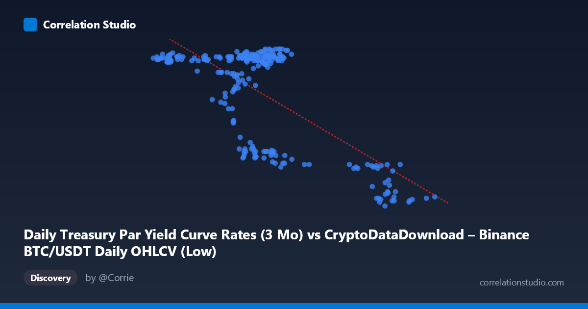
Daily Treasury Par Yield Curve Rates (3 Mo) vs CryptoDataDownload – Binance BTC/USDT Daily OHLCV (Low)
- Pearson correlation (r)
- -0.7003
- Spearman correlation
- -0.341
- p-value
- 0
- Sample size (n)
- 250
- 95% confidence interval
- -0.7584 to -0.631
- Granger causality
- None
- Granger optimal lag
- 1
AI analysis
Analysis of Treasury 3-Month Yield vs. BTC/USDT Daily Low
1. Overview of the Relationship
The scatterplot displays a clear negative relationship between the two variables (mislabeled axes aside — the analysis proceeds using the statistics provided). As the X variable increases, the Y variable declines, with the data forming two loosely defined clusters rather than a single continuous cloud: one dense grouping around X = 55,000–68,000 with Y values mostly between 5.2–5.5, and a second, sparser grouping at higher X values (85,000–105,000) with Y compressed into a narrow band around 4.3–4.6. This bimodal clustering suggests the relationship may be driven by two distinct regimes rather than a smooth continuous decline.
2. Strength, Direction, and Statistical Confidence
The correlation coefficient (r = -0.70) indicates a moderately strong negative linear relationship. The r² of 0.49 means that only about 49% of the variance in Y is explained by X — a meaningful but incomplete relationship, leaving over half of Y's variability attributable to other factors, noise, or nonlinear dynamics not captured by this simple linear model. The 95% confidence interval [-0.7584, -0.6310] is fairly tight and does not cross zero, and the p-value of ~0 confirms this correlation is highly statistically significant and not a product of chance, given the sample size of 250. However, statistical significance and practical explanatory power are different things: while we can be confident a negative association exists, the linear model still leaves substantial unexplained variance. Critically, the Granger causality tests show no significant predictive direction in either direction (X→Y: p=0.25; Y→X: p=0.37). This means that despite the strong contemporaneous correlation, neither variable helps forecast future values of the other — the relationship appears to be a co-movement or shared-driver phenomenon rather than one variable temporally leading the other.
3. Notable Patterns and Clusters
The most striking feature is the apparent two-cluster structure: a "high-Y/mid-X" cluster and a "low-Y/high-X" cluster, with relatively few intermediate points bridging them. This creates a visual impression of a steep drop or step-like transition rather than a smooth linear decay, even though the aggregate linear fit produces a moderate negative slope. Within the primary cluster (X ≈ 55,000–68,000), Y values themselves split into two sub-bands — one near 5.4–5.5 and another near 4.6–5.0 — suggesting an additional latent variable or time-based regime shift affects Y independently of X in this range. This intra-cluster scatter is likely the main source of the unexplained variance (the other ~51%).
4. Confounding Factors and Caveats
Since this data pairs a Treasury yield curve rate with BTC/USDT OHLCV data, the "relationship" is almost certainly mediated by shared macroeconomic time trends rather than direct causation. Both series may be independently trending over the 2024 calendar year (e.g., Fed policy shifts affecting short-term yields, and separate crypto-market cycles affecting BTC), producing spurious correlation through common time-dependence rather than genuine interaction. The lack of Granger causality reinforces this concern — real causal or predictive linkages would typically show up as lead-lag structure, and none was found. Additionally, both series are non-stationary time series (trending rates, trending crypto prices), which is well known to inflate correlation coefficients artificially even absent causal linkage.
5. Suggested Next Steps
Analysts should first detrend or first-difference both series (converting to daily/period changes) and recompute correlation to test whether the relationship survives — this is the standard remedy for spurious trend-driven correlation. Segmenting the data by the two visible clusters (or by calendar quarter) and testing correlation within each regime separately would clarify whether the relationship is stable or an artifact of a single structural break (e.g., a rate hike/cut event or a crypto market shock coinciding with a particular period). Given the non-significant Granger results, this pairing should be treated as descriptive/correlational only — not used for forecasting one series from the other — and further work should look for shared external drivers (Fed policy announcements, risk-on/risk-off sentiment indices) that might jointly explain both series' movements more convincingly than a direct bivariate link.
X dataset: CryptoDataDownload – Binance BTC/USDT Daily OHLCV
Y dataset: Daily Treasury Par Yield Curve Rates
Part of experiment: Bitcoin - CryptoDataDownload – Binance BTC/USDT Daily OHLCV vs Daily Treasury Par Yield Curve Rates