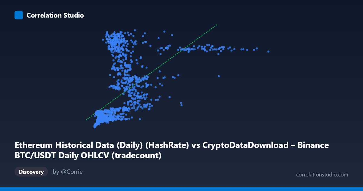
Ethereum Historical Data (Daily) (HashRate) vs CryptoDataDownload – Binance BTC/USDT Daily OHLCV (tradecount)
- Pearson correlation (r)
- 0.5862
- Spearman correlation
- 0.7217
- p-value
- 0
- Sample size (n)
- 1855
- 95% confidence interval
- 0.5555 to 0.6153
- Granger causality
- X → Y
- Granger optimal lag
- 2
AI analysis
Analysis of X-Y Relationship
1. What the visualization reveals
The scatterplot shows a positive but noisy relationship between the X variable (labeled here as "HashRate" but described in metadata as OHLCV price data) and Y (tradecount). Most points cluster at low X values (under ~2,000,000) with Y values spread widely between roughly 100 and 1000, while a smaller number of high-X outliers (2.4M–8.8M) also show generally elevated Y values. This creates a classic "fan" or "wedge" shape — tight clustering at low X with increasing scatter — rather than a clean linear band, which is consistent with the moderate r² value.
2. Strength, direction, and uncertainty
The correlation coefficient (r = 0.586) indicates a moderate positive linear relationship, but r² = 0.344 tells the more important story: only about 34% of the variance in Y is explained by X, leaving roughly two-thirds of Y's variability attributable to other factors or noise. The 95% CI [0.556, 0.615] is fairly narrow given the large sample (n=1,855), so we can be confident the true population correlation is moderate — not spurious — and the p-value of ~0 confirms statistical significance. However, statistical significance here reflects sample size more than practical strength; a moderate r² means X alone is a weak-to-moderate predictor of Y. The Granger causality results add a temporal dimension: X→Y is significant (p=0.029) while Y→X is not (p=0.084), suggesting X's past values help predict future Y beyond Y's own history — a unidirectional predictive relationship, though the effect (F≈3.6) is modest and lag is short (2 periods), so this should be treated as suggestive rather than proof of causal mechanism.
3. Notable patterns and outliers
Several high-Y outliers appear at relatively low-to-mid X values (e.g., X≈862,880 with Y≈1016; X≈423,446 with Y≈970; X≈616,536 with Y≈975), indicating that large tradecount spikes can occur independent of the X metric — likely tied to specific market events (volume surges, volatility spikes) rather than gradual scaling with X. Conversely, many low-Y points (Y<250) persist across a wide range of low X values, suggesting a floor/baseline tradecount unrelated to X until some threshold. The extreme X outliers (millions in magnitude, e.g., 8.86M) sit at the tail of the distribution (mean 979,699, stdev 1,174,590) and may exert disproportionate leverage on the regression line — worth checking via Cook's distance or leverage plots. The note that Spearman ρ exceeds Pearson r reinforces that the relationship's monotonic strength is understated by the linear model, pointing to curvature (possibly logarithmic or power-law) rather than a straight line.
4. Confounding factors and caveats
There's a significant metadata inconsistency: X is labeled "Ethereum Historical Data (HashRate)" but its source description references BTC/USDT OHLCV price/volume data, while Y (tradecount) is attributed to Ethereum network metrics. This suggests possible column mislabeling or a merged dataset where variable identities are unclear — a critical caveat before drawing any domain conclusions (e.g., "hashrate predicts tradecount"). Additionally, both crypto price/volume and network activity metrics are highly non-stationary time series (2017–2022) that trend upward together during bull markets — the correlation may partly reflect a shared temporal trend (both rising during 2020-2021 bull run) rather than a direct mechanical relationship. This is a classic confound in Granger causality testing on non-stationary series, which can produce spurious "causality" unless differencing or cointegration testing is applied.
5. Actionable insights
First, resolve the label/source ambiguity to confirm what X and Y actually represent before publishing conclusions. Second, test log-transforming X (given its extreme right skew, stdev mean) or Y, since a log-linear or power model may raise R² substantially given the Spearman/Pearson gap. Third, run stationarity tests (ADF) on both series and consider differencing before re-running Granger causality, since trending crypto series often generate false-positive directional signals. Finally, given the moderate r² and short optimal lag, treat the X→Y predictive signal as a weak leading indicator at best — useful perhaps as one input in a multivariate forecasting model, but not a standalone predictor of tradecount.
X dataset: CryptoDataDownload – Binance BTC/USDT Daily OHLCV
Y dataset: Ethereum Historical Data (Daily)
Part of experiment: Bitcoin - CryptoDataDownload – Binance BTC/USDT Daily OHLCV vs Ethereum Historical Data (Daily)