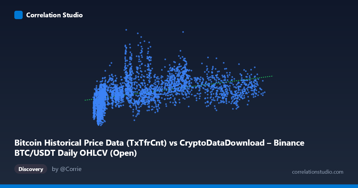
Bitcoin Historical Price Data (TxTfrCnt) vs CryptoDataDownload – Binance BTC/USDT Daily OHLCV (Open)
- Pearson correlation (r)
- 0.4341
- Spearman correlation
- 0.6005
- p-value
- 0
- Sample size (n)
- 3191
- 95% confidence interval
- 0.4055 to 0.4619
- Granger causality
- None
- Granger optimal lag
- 10
AI analysis
Analysis: Bitcoin Transaction Count vs. Opening Price
1. What the Visualization Reveals
The scatterplot shows a moderate positive relationship between Bitcoin's daily transaction count (X) and its opening price (Y). Points are diffusely scattered rather than tightly clustered along a line, indicating that while higher transaction counts tend to co-occur with higher prices, the relationship is loose and noisy. The data spans a wide X range (roughly 3,200 to 124,600 transactions) against a Y range of $365K to $1.68M, suggesting this covers multiple market cycles rather than a single trend period.
2. Strength, Direction, and Statistical Confidence
The Pearson correlation of r = 0.434 is a moderate positive relationship, but r² = 0.189 tells the more important practical story: transaction count explains less than 19% of the variance in price. The remaining ~81% is driven by other factors (macro sentiment, liquidity, halving cycles, etc.). The 95% CI [0.406, 0.462] is fairly tight given the large sample (n=3,191), and the p-value of ~0 confirms this correlation is statistically real, not due to chance — but statistical significance here reflects sample size more than practical strength.
Critically, the Granger causality tests show no significant predictive direction in either direction (X→Y: p=0.247; Y→X: p=0.921). This means neither transaction count nor price reliably leads the other in a time-series sense at the tested lag (10 periods). The correlation appears contemporaneous/associative rather than causal or predictive — likely both variables are driven by a shared underlying factor (overall market activity/adoption cycles) rather than one directly forecasting the other.
3. Notable Patterns and Non-linear Features
The sample points show a "wedge" or "fan" shape: at low transaction counts (~3,000–10,000), Y prices vary enormously (from ~$370K to ~$940K), while at higher transaction counts (80,000), price values compress into a narrower, higher band (~$830K–$1.05M). This heteroscedastic pattern — variance in Y decreasing as X increases — is a classic sign of a non-linear or logarithmic relationship, which aligns with the note that Spearman ρ exceeds Pearson r. A log or square-root transform of X would likely straighten the relationship and improve fit, consistent with diminishing marginal price sensitivity to added transaction volume.
4. Confounding Factors and Caveats
- Time-series autocorrelation: Both variables are trending series over ~9 years (2017–2026) covering bull/bear cycles; naive correlation on non-stationary time series can produce spurious associations. Detrending or differencing (returns/changes rather than levels) would give a more honest picture. - Shared external drivers: Broader market activity, exchange volume, media attention, and macro liquidity conditions likely drive both metrics simultaneously. - Structural breaks: Bitcoin's price history includes distinct regimes (2017 bubble, 2020-21 bull run, 2022 crash, etc.) that may each have different X-Y relationships, diluting a single linear fit. - Network growth confound: Transaction count naturally grows over time as adoption increases, independent of price — this secular trend could inflate correlation without genuine link.
5. Actionable Insights
- Model refinement: Apply a log transformation to X (transaction count) or fit a power/log curve instead of linear regression to better capture the diminishing-returns pattern. - Use returns, not levels: Re-run correlation and Granger tests on day-over-day % changes in both series to remove trend-driven spurious correlation and test genuine short-term dynamics. - Segment by regime: Split data into bull/bear/sideways market phases and re-analyze — the pooled r may mask stronger or weaker relationships within specific periods. - Explore other lags/variables: Given no Granger causality at lag 10, test shorter lags (1-5 days) or introduce a third variable (e.g., trading volume, active addresses) that may mediate the relationship. - Treat as descriptive, not predictive: Given the null Granger result, this correlation should not be used for trading signals or forecasting price from transaction counts — it's better suited for describing market activity co-movement.
X dataset: CryptoDataDownload – Binance BTC/USDT Daily OHLCV
Y dataset: Bitcoin Historical Price Data
Part of experiment: Bitcoin - CryptoDataDownload – Binance BTC/USDT Daily OHLCV vs Bitcoin Historical Price Data