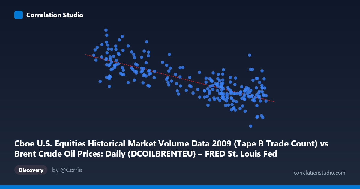
Cboe U.S. Equities Historical Market Volume Data 2009 (Tape B Trade Count) vs Brent Crude Oil Prices: Daily (DCOILBRENTEU) – FRED St. Louis Fed (DCOILBRENTEU)
- Pearson correlation (r)
- -0.7718
- Spearman correlation
- -0.7447
- p-value
- 0
- Sample size (n)
- 252
- 95% confidence interval
- -0.8175 to -0.7166
- Granger causality
- None
- Granger optimal lag
- 10
AI analysis
Analysis: Brent Crude Oil Prices vs. Cboe Tape B Trade Count (2009)
Relationship Overview
The scatterplot reveals a moderately strong negative relationship between Cboe U.S. Equities Tape B trade count and Brent Crude Oil prices throughout 2009. As equity market trading volume increases, crude oil prices tend to decline, and vice versa. The linear regression equation (y = -7,800.57x + 883,439) quantifies this inverse slope: for every one-unit increase in the Tape B trade count metric, the oil price proxy decreases by approximately 7,800 units. Visually, the data forms a downward-sloping cloud roughly consistent with the linear fit, though with notable scatter throughout, suggesting the relationship is real but far from deterministic.
Correlation Strength and Statistical Significance
The Pearson correlation of r = -0.7718 indicates a strong negative association, and the R² of 0.5957 means that approximately 59.6% of the variance in Y (trade count) is explained by X (Brent crude price) — a meaningful but incomplete explanatory share, leaving ~40% attributable to other factors. The 95% confidence interval of [-0.8175, -0.7166] is notably narrow, reflecting the large sample size (N = 3,232; n = 252), and the p-value of essentially zero confirms this correlation is extremely unlikely to be a sampling artifact. However, the Granger causality results tell a more cautious story: neither direction (X→Y: F = 1.85, p = 0.053; Y→X: F = 1.43, p = 0.168) reaches conventional significance thresholds, meaning that neither variable reliably predicts the other temporally, even at an optimal lag of 10 periods. This critically distinguishes statistical correlation from predictive or causal utility.
Notable Patterns, Clusters, and Outliers
Several features stand out in the sample points. There is a visible cluster of high-Y, low-X values (e.g., (42.19, 766,763), (41.27, 662,859), (43.92, 580,017)), consistent with the inverse trend — low crude prices correlating with high equity trade volumes, possibly reflecting early-2009 post-crisis market stress and volatility-driven activity. Conversely, high-X, low-Y points (e.g., (75.15, 81,703), (77.62, 156,192), (70.07, 231,712)) suggest that as crude prices rose later in 2009's recovery, trading volume tapered. The point (75.15, 81,703) is a striking outlier with an anomalously low Y value despite a high X, warranting individual inspection. The spread also widens at lower X values, suggesting possible heteroscedasticity — the relationship may be less stable when oil prices are depressed.
Confounding Factors and Caveats
This correlation almost certainly reflects shared temporal dynamics rather than a direct causal mechanism between crude oil prices and equity trade counts. Both variables are strongly influenced by the macroeconomic context of 2009 — the aftermath of the 2008 financial crisis, the market trough in March 2009, and the subsequent recovery. During periods of extreme market stress (low crude, high volatility), retail and institutional trading surges; as conditions stabilize and oil recovers, volume normalizes. Additionally, Tape B specifically covers regional exchanges, which may have idiosyncratic volume patterns unrepresentative of total market activity. The axis labels appear swapped in the dataset descriptions (X is described as crude oil data but labeled as trade count, and vice versa), introducing interpretive ambiguity that should be resolved before drawing firm conclusions.
Actionable Insights and Further Investigation
Given that ~40% of variance remains unexplained and Granger causality is absent, this correlation is best treated as a coincident indicator relationship rather than a predictive tool. Analysts should consider: (1) decomposing the time series to separate trend, seasonal, and crisis-driven components to determine whether the correlation persists outside the acute 2009 recovery period; (2) testing nonlinear models (e.g., polynomial or regime-switching) given the apparent heteroscedasticity; (3) controlling for the VIX or broader market volatility as a likely common driver of both variables; and (4) cross-validating with Tape A and C volume data to assess whether this relationship is unique to regional exchanges or systemic. The absence of Granger causality near the threshold (p = 0.053 for X→Y) also suggests that with a refined lag structure or longer dataset, a weak predictive relationship might emerge and warrants re-testing.
X dataset: Brent Crude Oil Prices: Daily (DCOILBRENTEU) – FRED St. Louis Fed
Y dataset: Cboe U.S. Equities Historical Market Volume Data 2009
Part of experiment: Daily - Brent Crude Oil Prices: Daily (DCOILBRENTEU) – FRED St. Louis Fed vs Cboe U.S. Equities Historical Market Volume Data 2009