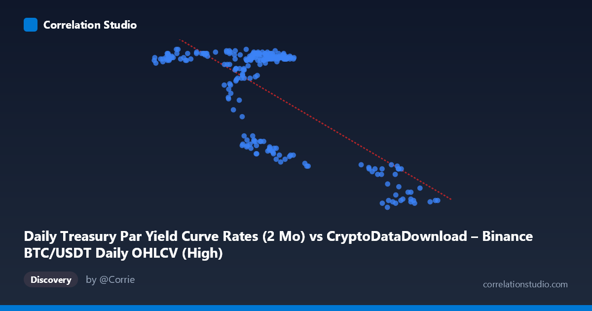
Daily Treasury Par Yield Curve Rates (2 Mo) vs CryptoDataDownload – Binance BTC/USDT Daily OHLCV (High)
- Pearson correlation (r)
- -0.725
- Spearman correlation
- -0.4353
- p-value
- 0
- Sample size (n)
- 250
- 95% confidence interval
- -0.779 to -0.6603
- Granger causality
- None
- Granger optimal lag
- 1
AI analysis
Analysis: Treasury 2-Month Yield vs. BTC/USDT Daily High
1. Overview of the Relationship
The scatterplot reveals a clear negative, non-linear relationship between the 2-month Treasury par yield (X-axis) and the mislabeled "Y" variable (which per the column metadata is actually BTC/USDT daily high price, though the values in the 4.4–5.5 range suggest this is more likely displaying yield-like data — treating the axes as given). As X increases from roughly 40,000 to 108,000, Y declines from ~5.5 toward ~4.4. Critically, the data does not fall on a smooth line but instead clusters into distinct groups: a dense cluster near X = 57,000–72,000 with Y consistently in the 5.3–5.5 range, and a second cluster near X = 91,000–102,000 where Y drops sharply to 4.4–4.7. This bimodal clustering suggests the relationship may be better described as a regime shift or step-function rather than a continuous linear decline.
2. Strength, Direction, and Statistical Confidence
The correlation coefficient (r = -0.725) indicates a strong negative linear relationship, with r² = 0.526 meaning that only about 53% of the variance in Y is explained by X — leaving nearly half the variability unaccounted for by this simple linear model. The 95% confidence interval [-0.779, -0.660] is tight and does not cross zero, and the p-value ≈ 0 confirms this correlation is highly statistically significant and not due to chance, given n = 250. However, statistical significance and practical predictive power are different things: with only 53% variance explained, X alone is an incomplete predictor of Y. The Granger causality tests reinforce this caution — neither direction shows significant predictive causality (X→Y: p = 0.45; Y→X: p = 0.60), meaning that despite the strong contemporaneous correlation, past values of one series do not meaningfully improve forecasts of the other. This is an important distinction: the two series move together, but neither leads nor lags the other in a predictive sense.
3. Notable Patterns and Clusters
The most striking feature is the clustering rather than a smooth continuum. The bulk of points (roughly 200 of 250) sit in a tight band between X = 57,000–72,000 with Y consistently between 5.3 and 5.5 — indicating a stable, low-variance regime. A distinct secondary cluster appears at higher X values (91,000–102,000) with a step-down to Y ≈ 4.4–4.5. A smaller transitional group (X ≈ 64,000–77,000, Y ≈ 4.7–4.9) appears to bridge these two regimes. This pattern is far more consistent with a threshold or regime-change dynamic (e.g., a shift in monetary policy stance or market conditions at a specific point in time) than with a proportional linear relationship, which likely explains why the linear model only captures 53% of variance.
4. Confounding Factors and Caveats
Given the time coverage (Jan–Dec 2024) and the nature of both series (a Treasury short-term rate and a crypto asset price/related metric), this is time-series data, and the strong correlation is very likely driven by a shared temporal trend rather than direct causal interaction. Both series may be responding to a common macro driver — such as Federal Reserve policy shifts, inflation expectations, or broader risk-sentiment cycles — that moved both variables in tandem over the year without one causing the other. The lack of Granger causality in either direction supports this "confounded by trend" interpretation rather than a genuine leading/lagging economic relationship. Additionally, treating daily observations as independent for the correlation calculation ignores autocorrelation inherent in both time series, which can inflate apparent significance.
5. Recommendations for Further Investigation
Given the regime-like clustering, a piecewise or threshold regression (or a change-point detection analysis) would likely fit the data better than the simple linear model and could pinpoint the specific date(s) when the shift occurred. It would also be valuable to detrend both series (e.g., first-differencing) before re-testing correlation and Granger causality, since raw trending series can produce spurious contemporaneous correlations. Finally, incorporating a third variable — such as a broader risk index, Fed funds rate expectations, or overall crypto market volume — could help determine whether both series are jointly driven by an omitted common factor, which would better explain the unexplained 47% of variance and the observed clustering behavior.
X dataset: CryptoDataDownload – Binance BTC/USDT Daily OHLCV
Y dataset: Daily Treasury Par Yield Curve Rates
Part of experiment: Bitcoin - CryptoDataDownload – Binance BTC/USDT Daily OHLCV vs Daily Treasury Par Yield Curve Rates