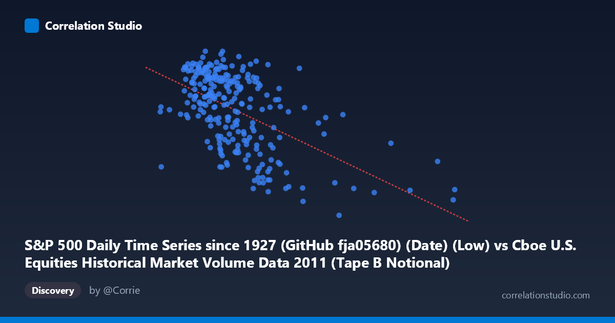
S&P 500 Daily Time Series since 1927 (GitHub fja05680) (Date) (Low) vs Cboe U.S. Equities Historical Market Volume Data 2011 (Tape B Notional)
- Pearson correlation (r)
- -0.5502
- Spearman correlation
- -0.5084
- p-value
- 0
- Sample size (n)
- 252
- 95% confidence interval
- -0.6309 to -0.4578
- Granger causality
- None
- Granger optimal lag
- 4
AI analysis
Analysis: S&P 500 Low Price vs. Cboe Tape B Notional Volume (2011)
Relationship Overview The scatterplot reveals a moderate negative relationship between the S&P 500 daily low price (X-axis) and Cboe Tape B notional trading volume (Y-axis) across 252 trading days in 2011. As the S&P 500 low price increases, Tape B notional volume tends to decrease. This inverse pattern is intuitive in context: during the 2011 market stress period (which included the U.S. debt ceiling crisis and European sovereign debt fears), prices were depressed while trading activity surged — and conversely, calmer, higher-price periods saw relatively subdued volume. The linear regression equation (y = -2.02×10⁻⁸x + 1360.62) captures this downward slope, though the scatter around the line is considerable.
Correlation Strength and Statistical Significance The Pearson correlation of r = -0.5502 indicates a moderate negative association, with r² = 0.3028 meaning that approximately 30.3% of the variance in Tape B notional volume is explained by variation in the S&P 500 low price. While statistically meaningful, this also means nearly 70% of variance remains unexplained by this relationship alone, underscoring that many other forces drive notional volume. The 95% confidence interval of [-0.6309, -0.4578] is relatively tight and does not cross zero, and the p-value is effectively zero, confirming the correlation is highly unlikely to be a chance artifact given n = 252 paired observations drawn from a population of N = 3,780. However, Granger causality tests reveal no significant predictive directionality in either direction (X→Y: F = 1.88, p = 0.11; Y→X: F = 0.20, p = 0.94) at the optimal lag of 4 periods. This is a critical caveat: while the two variables co-move, neither reliably predicts the other temporally, suggesting the relationship is contemporaneous and likely driven by shared underlying conditions rather than a lead-lag dynamic.
Notable Patterns, Clusters, and Outliers The sample points reveal several important structural features. There is a visible cluster of high-volume observations (Tape B Notional ~1,300–1,355) concentrated at lower S&P 500 low prices (roughly 3.0B–5.5B range on X), consistent with the volatile August–October 2011 correction period. Conversely, points with higher X values (prices above ~7B–10B) tend to cluster at lower notional volumes (~1,100–1,250), suggesting quieter late-year or early-year sessions. Several notable outliers are visible at very high X values (e.g., ~9.5B–14.1B) with relatively low Tape B notional values around 1,121–1,249, which may represent unusually low-activity high-price days. The distribution also shows heteroscedasticity — the vertical spread of Y values appears wider in the mid-range of X than at the extremes — which slightly undermines the assumptions of simple linear regression.
Confounding Factors and Caveats Several important caveats apply. First, 2011 was an exceptional year for U.S. equity markets, featuring multiple discrete volatility episodes (debt ceiling, S&P U.S. credit downgrade in August, European contagion fears), which means the negative correlation may be regime-specific and not generalizable to other years. Second, the X-axis label describes the S&P 500 daily low — a measure of intraday stress — rather than closing price or volume, which conflates price level with intraday volatility. Third, Tape B specifically covers NYSE American (AMEX) and regional exchange listings, so this is not broad market volume but a subset, and its behavior may diverge from total market volume dynamics. Fourth, the moderate r² suggests substantial omitted variable bias — factors such as VIX levels, macro news events, options expiration cycles, or algorithmic trading patterns likely explain much of the residual variance. The lack of Granger causality further reinforces that this correlation reflects common exposure to market stress rather than a structural or directional mechanism.
Actionable Insights and Further Investigation Practitioners should resist interpreting this relationship as a trading signal given the absence of Granger causality and the modest explanatory power. Instead, both variables likely serve as co-indicators of market stress regimes, making them potentially useful together in a broader market condition classification model (e.g., distinguishing high-stress from low-stress trading environments). Further investigation should include: (1) segmenting the data by volatility regime (e.g., using VIX quartiles) to test whether the correlation strengthens during stress periods; (2) expanding to multiple years to test whether the negative relationship persists or is 2011-specific; (3) incorporating total market notional volume rather than Tape B alone to assess whether this is a broad-market or exchange-specific phenomenon; and (4) applying non-linear modeling (e.g., piecewise regression or LOESS smoothing) given the apparent heteroscedasticity and clustering, as the true relationship may not be adequately captured by a linear fit.
X dataset: Cboe U.S. Equities Historical Market Volume Data 2011
Y dataset: S&P 500 Daily Time Series since 1927 (GitHub fja05680) (Date)
Part of experiment: Daily - Cboe U.S. Equities Historical Market Volume Data 2011 vs S&P 500 Daily Time Series since 1927 (GitHub fja05680) (Date)