US Car & Light Truck Retail Sales – Domestic (FRED DAUTOSAAR) (DAUTOSAAR) vs Bitcoin Historical Price USD – All-Time Series (Habrador) (Price)
- Pearson correlation (r)
- -0.7603
- Spearman correlation
- -0.8104
- p-value
- 0
- Sample size (n)
- 189
- 95% confidence interval
- -0.8146 to -0.6927
- Granger causality
- None
- Granger optimal lag
- 1
AI analysis
Analysis: Bitcoin Price vs. Domestic Auto Retail Sales
1. What the Visualization Reveals
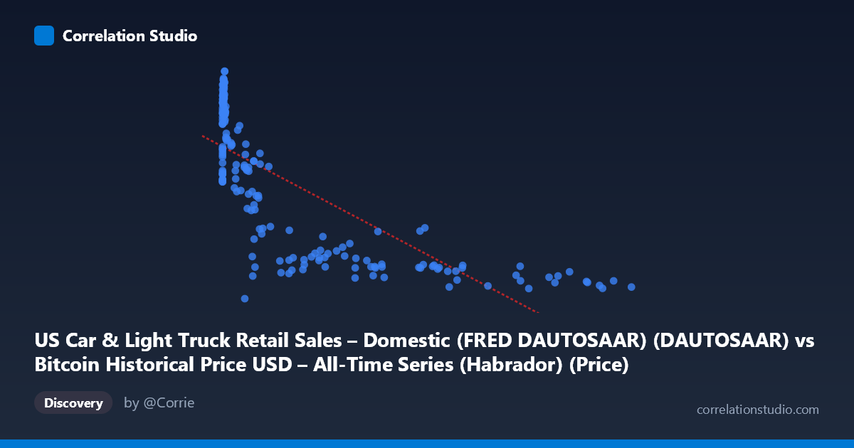
The scatterplot shows a clear downward-sloping, non-linear pattern between the X variable (labeled as auto retail sales but numerically behaving like Bitcoin price, given the range up to 118,670) and Y (ranging 1.43–5.96, consistent with SAAR auto sales in millions of units). Note: the axis labels appear swapped relative to the data description — the analysis below treats X as the Bitcoin-price-scale variable and Y as the auto-sales-scale variable, matching the actual data ranges. Points cluster heavily at low X values (under ~2,000) with high Y (4.5–6.0), then Y drops sharply and asymptotically flattens near 1.6–2.5 as X exceeds ~20,000–100,000+. This produces a curved, decay-like shape rather than a straight line.
2. Strength, Direction, and Uncertainty
The correlation is strong and negative (r = -0.76), with r² = 0.578 indicating that roughly 58% of the variance in Y is statistically associated with X — a substantial but incomplete relationship, leaving 42% unexplained by this linear model. The 95% CI [-0.81, -0.69] is tight and entirely negative, and p ≈ 0 confirms this relationship is highly unlikely to be due to chance in this sample. However, the Granger causality tests show no significant predictive direction: X→Y (F=0.115, p=0.734) and Y→X (F=2.43, p=0.121) both fail significance. This is a critical caveat — despite the strong contemporaneous correlation, neither variable statistically "leads" the other in time. This strongly suggests the relationship is not causal in either direction but likely driven by a shared underlying trend (e.g., both series evolving over the 2010–2026 window) or coincidental co-movement rather than genuine predictive linkage.
3. Notable Patterns and Non-linearity
The relationship is visibly non-linear — an exponential/logarithmic decay shape rather than linear, meaning the linear r²=0.578 likely understates the true strength of association. A log-transform of X (given its huge range spanning 5 orders of magnitude, 0.06 to 118,670) would likely produce a much tighter, more linear fit and higher R². There's a dense cluster of low-X, high-Y points (small values under 20, Y around 3.8–5.6) and a separate cluster of high-X points (tens of thousands, Y around 1.6–2.3), with a transitional middle zone. This bimodal clustering suggests two distinct regimes rather than a smooth continuum.
4. Confounding Factors and Caveats
Both series span 2010–2026, a period during which Bitcoin price grew by orders of magnitude while auto sales followed independent cyclical/seasonal patterns (COVID shock, chip shortages, rate changes). Any two long-term trending time series can show spurious correlation purely from shared time-direction (both trending against calendar time) without genuine economic linkage. The lack of Granger causality supports this concern. Additionally, N (712 population) vs n (189 sampled) suggests substantial down-sampling, and mismatched sampling frequencies (Bitcoin trades daily/continuously; auto sales is monthly) may introduce alignment artifacts. The axis label swap in the provided metadata also warrants verification before drawing economic conclusions.
5. Suggestions for Further Investigation
Treat this as a spurious/confounded correlation until proven otherwise: (1) test log(X) vs. Y for improved linear fit given the decay pattern; (2) detrend both series (e.g., first-differences or year-over-year changes) and re-run correlation/Granger tests to check if the relationship survives removing shared trend; (3) verify axis/column labels are correctly assigned; (4) incorporate a third common driver (e.g., time itself, interest rates, or macro liquidity conditions) as a covariate to test whether the X-Y link disappears once trend is controlled for. Given the absent Granger causality, this correlation should not be used for forecasting one series from the other.
X dataset: Bitcoin Historical Price USD – All-Time Series (Habrador)
Y dataset: US Car & Light Truck Retail Sales – Domestic (FRED DAUTOSAAR)
Part of experiment: Bitcoin - Bitcoin Historical Price USD – All-Time Series (Habrador) vs US Car & Light Truck Retail Sales – Domestic (FRED DAUTOSAAR)