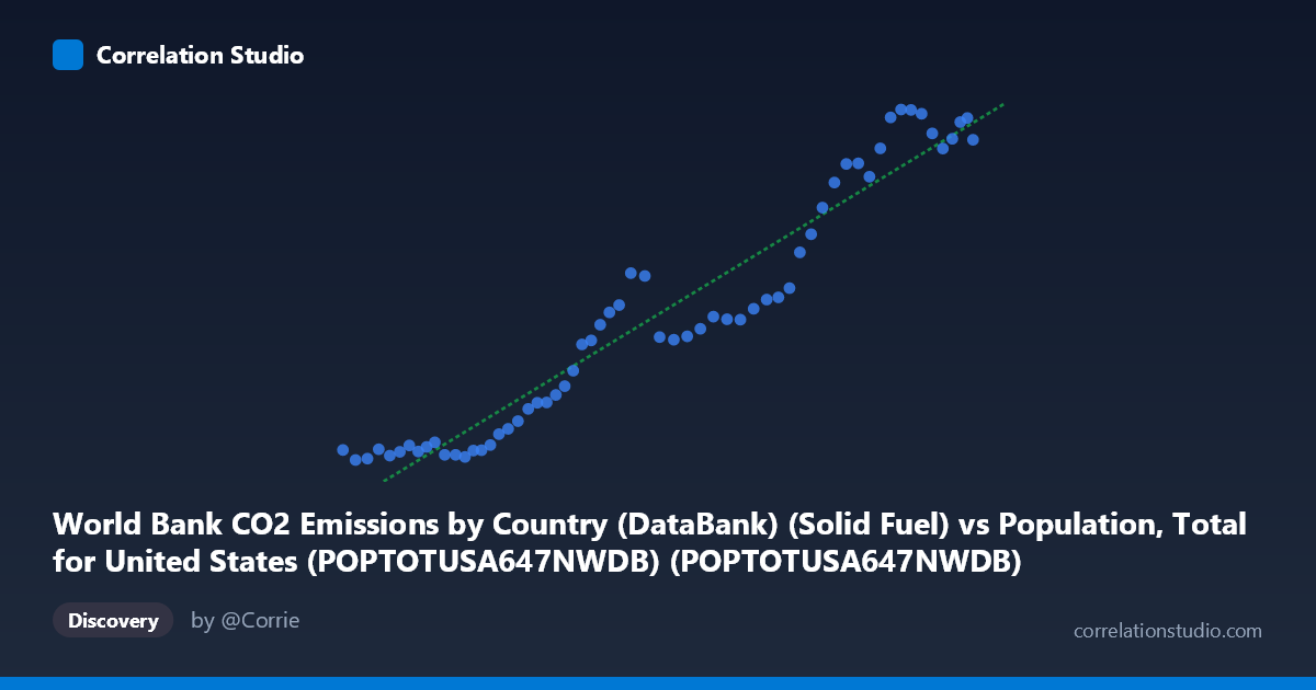
World Bank CO2 Emissions by Country (DataBank) (Solid Fuel) vs Population, Total for United States (POPTOTUSA647NWDB) (POPTOTUSA647NWDB)
- Pearson correlation (r)
- 0.964
- Spearman correlation
- 0.9646
- p-value
- 0
- Sample size (n)
- 61
- 95% confidence interval
- 0.9405 to 0.9783
- Granger causality
- None
- Granger optimal lag
- 10
- Time coverage
- 1960-01-01 to 2020-01-01
AI analysis
Scatterplot Analysis: U.S. Population vs. CO₂ Solid Fuel Emissions (1960–2020)
1. Overall Relationship
The scatterplot reveals a strong, predominantly positive relationship between total U.S. population and CO₂ emissions from solid fuels over the 1960–2020 period. As population grows from roughly 181 million to 332 million, solid fuel CO₂ emissions rise from approximately 12,300 to 31,200 units (likely thousand metric tons). The linear regression equation (y = 0.000136x − 14,812) captures this upward trajectory well, though the scatter around the fitted line is not perfectly uniform across the full range, suggesting the relationship may carry some structural nuance beyond a simple linear form.
2. Correlation Strength, Direction, and Causality
The Pearson correlation of r = 0.9640 indicates a very strong positive association, and the R² = 0.9293 means that approximately 92.9% of the variance in solid fuel CO₂ emissions is statistically explained by U.S. population size — a remarkably high figure for real-world socioeconomic data. The 95% confidence interval for r [0.9405, 0.9783] is narrow and entirely in the high-positive range, confirming this is not a chance finding, and the p-value of effectively zero (p ≈ 0) rules out sampling error as an explanation for the observed association. However, Granger causality tests complicate the causal narrative significantly: neither direction (X→Y nor Y→X) reaches statistical significance at the optimal lag of 10 periods (X→Y: F = 1.43, p = 0.21; Y→X: F = 1.57, p = 0.16). This means that, in a temporal sense, knowing population today does not reliably help predict future CO₂ emissions beyond what CO₂ itself already predicts, and vice versa — both variables are likely co-evolving along a shared third trajectory (time/economic growth) rather than one directly driving the other.
3. Patterns, Clusters, and Notable Features
Visually, the data points cluster into at least two distinct behavioral zones. The lower-left cluster (population ~181–240 million, emissions ~12,300–18,000) spans roughly the 1960s through mid-1980s and shows a relatively tight, steep upward progression. A transitional middle zone (population ~240–285 million) displays somewhat more scatter, with emissions ranging broadly from ~18,500 to ~24,500, hinting at a period of decoupling or efficiency gains. The upper-right cluster (population ~295–332 million, emissions ~25,000–31,150) shows high emissions values but also some compression — several high-population points have notably similar emission levels, possibly reflecting plateauing solid fuel use in recent decades. No dramatic outliers are evident, but points like (314M population, 31,154 emissions) and (316M, 31,132) stand out as the emission ceiling values, while (183M, 12,325) anchors the lower bound cleanly.
4. Confounding Factors and Caveats
The dominant caveat here is spurious correlation driven by shared temporal trend. Both U.S. population and CO₂ emissions from solid fuels are time-indexed variables that generally increase over the 20th century; their high correlation may reflect little more than the fact that both trend upward over time (a classic "third variable" problem where time is the true driver). The Granger causality failure directly supports this interpretation. Additional confounders include: economic growth and industrialization (GDP likely mediates both); energy policy shifts (coal regulations, Clean Air Act amendments, and the shale gas revolution post-2005 reduced coal use while population kept growing); technological efficiency changes (emissions per capita and per unit GDP have changed substantially); and the specific metric of "solid fuel" emissions, which tracks coal and similar sources rather than total fossil fuel use, making it sensitive to fuel-switching dynamics that are independent of population. The linear model's assumption of a constant per-person emission rate (the slope) is also likely violated across such a long timeframe.
5. Actionable Insights and Further Investigation
Given the high R² but absent Granger causality, the most productive next steps would be to partial out the time trend (e.g., first-differencing both series or detrending with a cubic spline) and re-examine whether any residual correlation persists — this would test whether population changes predict emission changes beyond shared momentum. Researchers should also decompose emissions by sector (residential, industrial, power generation) to identify which components track population most closely versus those driven by industrial or energy-market dynamics. A per-capita emissions analysis would be particularly revealing: if per-capita solid fuel emissions are declining while total emissions correlate with population, the story is one of efficiency gains being outpaced by population growth rather than population "causing" emissions. Finally, extending the analysis to include GDP, energy price indices, and policy event markers (e.g., Clean Power Plan, major coal plant retirements) as covariates in a multivariate regression would help isolate the independent contribution of population, and a cross-country comparison using the World Bank dataset would test whether the U.S. pattern generalizes or reflects country-specific structural features.
X dataset: Population, Total for United States (POPTOTUSA647NWDB)
Y dataset: World Bank CO2 Emissions by Country (DataBank)
Part of experiment: Yearly - Population, Total for United States (POPTOTUSA647NWDB) vs World Bank CO2 Emissions by Country (DataBank)