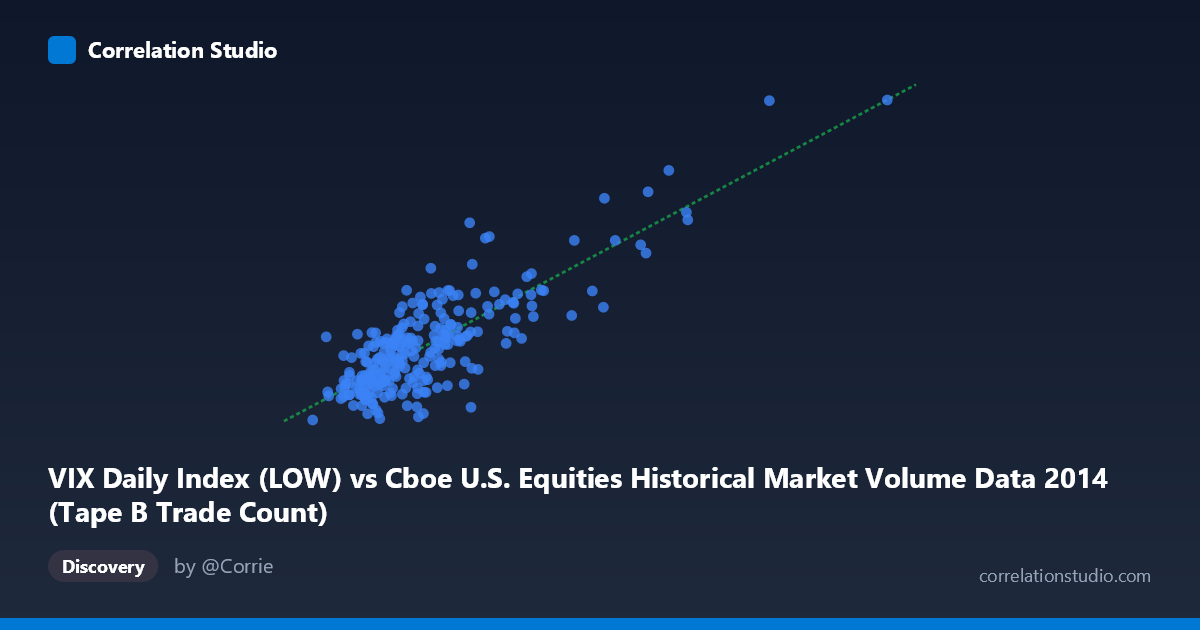
VIX Daily Index (LOW) vs Cboe U.S. Equities Historical Market Volume Data 2014 (Tape B Trade Count)
- Pearson correlation (r)
- 0.8173
- Spearman correlation
- 0.6993
- p-value
- 0
- Sample size (n)
- 252
- 95% confidence interval
- 0.7717 to 0.8546
- Granger causality
- None
- Granger optimal lag
- 1
AI analysis
Analysis: VIX Low vs. Tape B Trade Count (2014)
Relationship Overview The scatterplot reveals a moderately strong positive relationship between the VIX Daily Index Low values and the Cboe U.S. Equities Tape B Trade Count across 2014. As the VIX low increases — indicating rising baseline market volatility — the number of Tape B trades tends to increase meaningfully. The linear regression equation (y = 2.43e-05x + 8.23) suggests that for every 100,000-unit increase in the VIX low, trade count rises by approximately 2.43 units, though the practical interpretation requires careful attention to scale and units. The relationship appears broadly linear across the moderate range of the data, with notable deviations at the upper extremes of X.
Correlation Strength and Statistical Significance The Pearson correlation of r = 0.8173 indicates a strong positive association, and the R² of 0.668 means that roughly 66.8% of the variance in Tape B trade counts is explained by the VIX low level — a substantial explanatory share, though one-third of variance remains attributable to other factors. The 95% confidence interval of [0.772, 0.855] is relatively narrow given the sample size of 252, lending considerable precision to this estimate, and the p-value of effectively zero confirms this is not a chance finding. However, despite the strong contemporaneous correlation, the Granger causality tests are non-significant in both directions (X→Y: F = 1.78, p = 0.18; Y→X: F = 0.05, p = 0.82), meaning neither variable reliably predicts the future values of the other at a one-period lag. This is a critical distinction: the variables move together, but neither demonstrably leads the other in a temporal sense, cautioning against causal interpretations.
Patterns, Clusters, and Outliers The sample points reveal a dense cluster concentrated in the lower-left region, roughly where X falls between 110,000 and 280,000 and Y between 10 and 16 — reflecting the majority of 2014's relatively calm market environment. A smaller but visually striking group of points extends into the upper-right, with two particularly notable outliers near (559,868, 24.61) and (478,251, 19.60), which likely correspond to periods of acute volatility spikes (e.g., the October 2014 market selloff). These high-leverage points exert considerable influence on the regression line and correlation coefficient, and the spread of Y values at moderate X levels hints at mild heteroscedasticity — variance in trade counts appears to widen as VIX low increases.
Confounding Factors and Caveats Several important caveats apply. First, common-cause confounding is plausible: macroeconomic shocks or specific market events in 2014 (e.g., geopolitical tensions, Fed policy announcements) could simultaneously drive both elevated volatility and higher trade volumes without a direct causal link between them. Second, Tape B specifically covers NYSE American and regional exchanges, so the trade count reflects a subset of total market activity that may respond differently to volatility than the broader market. Third, the dataset is limited to a single calendar year, which constrains generalizability — 2014 was characterized by episodic volatility spikes against a generally low-volatility backdrop, and results could differ substantially in a sustained high-volatility regime. Finally, the non-significant Granger results at lag 1 may mask relationships at longer lags that were not tested.
Actionable Insights and Further Investigation Practitioners could use the contemporaneous relationship (R² ≈ 0.67) as a nowcasting signal: elevated VIX lows are associated with meaningfully higher Tape B trading activity, which has implications for exchange capacity planning, liquidity provision, and transaction cost modeling. To deepen this analysis, it would be worthwhile to: (1) test Granger causality at multiple lags (2–10 periods) to detect delayed predictive relationships; (2) segment the data by volatility regime (e.g., VIX < 15 vs. VIX 20) to assess whether the linear relationship holds uniformly or breaks down at extremes; (3) include additional covariates such as overall S&P 500 returns, macro announcements, or total market volume to disentangle the partial contribution of VIX to trade counts; and (4) replicate across multiple years to assess whether 2014's episodic volatility structure is driving the correlation or whether it represents a stable structural relationship.
X dataset: Cboe U.S. Equities Historical Market Volume Data 2014
Y dataset: VIX Daily Index
Part of experiment: Daily - Cboe U.S. Equities Historical Market Volume Data 2014 vs VIX Daily Index