Ethereum Historical Price Data (FlowOutExUSD) vs CryptoDataDownload – Binance BTC/USDT Daily OHLCV (Open)
- Pearson correlation (r)
- 0.6602
- Spearman correlation
- 0.8247
- p-value
- 0
- Sample size (n)
- 3191
- 95% confidence interval
- 0.6401 to 0.6793
- Granger causality
- Y → X
- Granger optimal lag
- 10
AI analysis
Analysis: Ethereum FlowOutExUSD vs. BTC/USDT Open Price
1. Overall Relationship
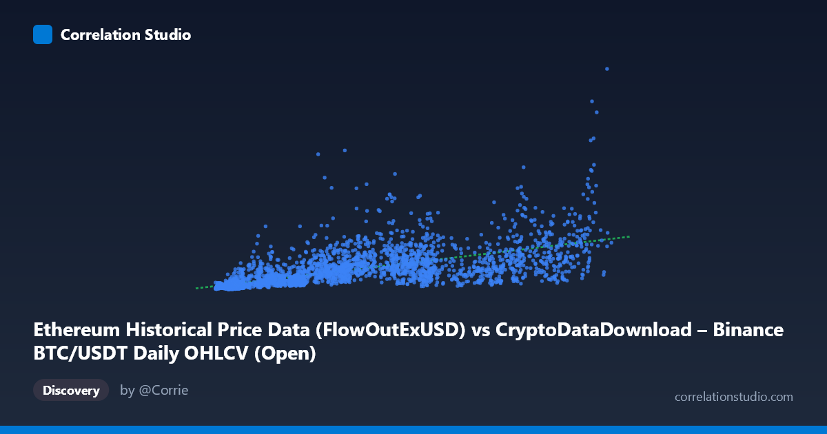
The scatterplot shows a positive, moderately strong association between the two variables: as the X-value (Ethereum's FlowOutExUSD) increases, the Y-value (BTC/USDT Open price) tends to rise as well. The data cloud is fairly wide, with substantial vertical scatter at almost every X level, indicating a real but noisy relationship rather than a tight linear one. The linear fit (y = 12,959.4x + 82.23M) captures the general upward trend but clearly doesn't account for a large share of the point-to-point variability, especially in the mid-to-high X range where Y values span an order of magnitude (e.g., X≈57,000 corresponds to Y values ranging from ~780M to ~1.69B across different samples).
2. Strength, Direction, and Statistical Confidence
The Pearson correlation (r = 0.66) indicates a moderate-to-strong positive linear relationship, but r² = 0.436 means only about 44% of the variance in Y is explained by X — the majority of Y's movement (56%) is driven by other factors not captured by this bivariate relationship. The 95% CI [0.640, 0.679] is tight, and the p-value is effectively 0, so we can be confident the correlation is real and not a sampling artifact — but statistical significance here reflects the large sample size (n=3,191) more than it reflects practical predictive strength. The Granger causality results add an important temporal dimension: X does not Granger-cause Y (p=0.143), but Y Granger-causes X at a 10-period lag (p=0.028, F=2.01). This suggests that past values of Y (BTC price) have some predictive power over future values of X (ETH outflow), rather than the reverse — the opposite of what one might intuitively assume from an "on-chain activity drives price" narrative.
3. Notable Patterns and Non-Linearity
The note that Spearman ρ exceeds Pearson r is a strong signal of non-linearity or heteroscedasticity in the data. Visually, this likely manifests as a fan-shaped or curved cloud — variance in Y increases substantially as X increases (heteroscedasticity), and the relationship may better resemble a power-law or logarithmic curve than a straight line. Several sample points stand out as high-leverage outliers relative to the linear trend: e.g., (14210, 702977435) has unusually high Y for very low X, and (40680.9, 1307766450) and (56425, 1395214518) show Y-values far above what the regression line predicts for their X. These suggest episodic spikes — possibly during high-volatility market events (bull runs, crashes) — where BTC price surges independently of ETH flow metrics, breaking the simple linear pattern.
4. Confounding Factors and Caveats
This is a classic case where two crypto-market series are compared across a shared multi-year window (2017–2026) that includes several major bull/bear cycles. Both BTC price and ETH exchange flows are likely driven by common macro factors — overall crypto market sentiment, liquidity cycles, regulatory news, and Bitcoin's own price dynamics (which heavily influence altcoin behavior including ETH) — making this a probable case of confounding rather than direct causation. The mismatch in dataset descriptions (X labeled as an Ethereum flow metric but sourced from "BTC/USDT" column, Y labeled from BTC OHLCV but described as "Ethereum" data) also raises a data-integrity concern — verify the column-to-dataset mapping before drawing firm conclusions, since axis mislabeling could seriously distort interpretation. Additionally, both series likely exhibit trends and autocorrelation over time (non-stationarity), which can inflate correlation coefficients and Granger test statistics independent of any real short-term causal linkage.
5. Suggestions for Further Investigation
Given the non-linearity signal, refit using log-transformed X and/or Y (or a power/polynomial model) and compare R² to the linear baseline. Detrend or difference both series (e.g., use returns/percentage changes rather than levels) before rerunning correlation and Granger tests to rule out spurious correlation from shared trends. Segment the analysis by market regime (bull vs. bear periods) to see if the relationship strength or direction changes. Finally, double-check data provenance/labeling given the apparent BTC/ETH column mismatch, and consider adding a third variable (e.g., overall market cap or trading volume) to test whether the observed correlation collapses once a common driver is controlled for.
X dataset: CryptoDataDownload – Binance BTC/USDT Daily OHLCV
Y dataset: Ethereum Historical Price Data
Part of experiment: Bitcoin - CryptoDataDownload – Binance BTC/USDT Daily OHLCV vs Ethereum Historical Price Data