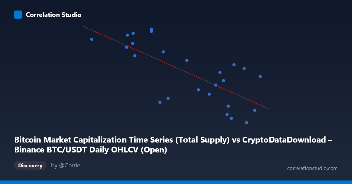
Bitcoin Market Capitalization Time Series (Total Supply) vs CryptoDataDownload – Binance BTC/USDT Daily OHLCV (Open)
- Pearson correlation (r)
- -0.7235
- Spearman correlation
- -0.7131
- p-value
- 0.000044
- Sample size (n)
- 25
- 95% confidence interval
- -0.8699 to -0.4597
- Granger causality
- None
- Granger optimal lag
- 6
- Time coverage
- 2024-03-29 to 2024-04-22
AI analysis
Analysis: Bitcoin Market Cap vs. BTC/USDT Opening Price
1. Overview of the Relationship
The scatterplot depicts 25 paired daily observations spanning late March to late April 2024, plotting Bitcoin's market capitalization (total supply basis) against the BTC/USDT opening price. Despite both variables nominally tracking "Bitcoin's value," the visualization reveals a negative relationship: as the market cap metric increases, the recorded opening price tends to decrease. This is counterintuitive at first glance, since market cap and price are typically mechanically linked (market cap = price × circulating supply), suggesting the two series may be capturing different underlying signals, timing conventions, or units (e.g., market cap in total supply terms vs. price at open, possibly from different snapshot times or slightly offset trading days).
2. Strength, Direction, and Statistical Confidence
The correlation coefficient of r = -0.7235 indicates a moderately strong negative linear relationship. The r² = 0.5234 tells us that roughly 52% of the variance in the Y-variable (opening price) is statistically explained by variance in the X-variable (market cap), leaving nearly half unexplained by this simple linear model — a meaningful but incomplete relationship. The 95% confidence interval [-0.8699, -0.4597] is comfortably bounded away from zero, and the p-value (4.377E-05) is highly significant, giving strong confidence that this negative association is not due to random chance in this sample. However, the Granger causality tests reveal no significant predictive direction in either direction (X→Y: p=0.4536; Y→X: p=0.1633) at the tested lag structure (optimal lag = 6 periods). This is an important distinction: the two series move together contemporaneously, but neither reliably forecasts future movements in the other over this 25-day window — the relationship appears associative/correlational rather than temporally predictive.
3. Patterns, Clusters, and Outliers
Visually, points cluster into two loose groups: a lower-X, higher-Y cluster (market cap ~61,000–65,000 range paired with prices near 19,682,000–19,688,000) and a higher-X, lower-Y cluster (market cap ~69,000–71,600 paired with prices near 19,667,000–19,681,000). This bimodal clustering suggests the data may reflect two distinct short-term regimes or trends within the sampling window rather than a single smooth linear relationship — consistent with Bitcoin's tendency to move in short trending phases. A few points (e.g., the extreme X value at 71,620 with a mid-range Y, and the lowest-X point at 61,277 with a relatively high Y) sit near the edges of the cloud and could exert outsized leverage on the regression slope. No strong evidence of a curved (non-linear) pattern is apparent, but with only 25 points, subtle non-linearities are hard to distinguish from noise.
4. Confounding Factors and Caveats
Several caveats warrant attention. First, the two "datasets" nominally describe the same underlying asset (Bitcoin) but sourced with different methodologies (market cap from an on-chain/supply-based series, price from Binance OHLCV) — misalignment in timestamps, exchange-specific pricing versus aggregated market data, or supply-count assumptions could introduce artificial divergence and even sign-flips in correlation. Second, with only 25 daily points over roughly one month, the sample is short relative to Bitcoin's typical volatility cycles, making the correlation vulnerable to short-term trend artifacts (e.g., a broad price decline coinciding with supply/market-cap increases) rather than a stable structural relationship. Third, autocorrelation within each time series (both are trending, non-stationary series) can inflate apparent correlation strength — this is a classic spurious-regression risk with financial time series and should be addressed via differencing or detrending before drawing causal conclusions.
5. Suggestions for Further Investigation
To validate and extend these findings: (1) re-run the correlation on differenced or percentage-change series rather than levels, to control for shared trends/non-stationarity and test whether the negative relationship persists; (2) verify data alignment — confirm both series reference the same timestamp convention (open vs. close, UTC vs. exchange time) and reconcile market cap's supply assumptions with actual circulating supply on those dates; (3) extend the sample window beyond 25 days to test whether the two apparent clusters represent a genuine regime shift or merely short-term noise; (4) given the lack of Granger causality, avoid using either series to forecast the other in a trading strategy without further lag testing (varying lag lengths, testing stationarity via ADF tests first); and (5) consider a multivariate model incorporating volume or volatility as additional explanatory variables, since 48% of variance remains unexplained by this bivariate relationship alone.
X dataset: CryptoDataDownload – Binance BTC/USDT Daily OHLCV
Y dataset: Bitcoin Market Capitalization Time Series
Part of experiment: Bitcoin - CryptoDataDownload – Binance BTC/USDT Daily OHLCV vs Bitcoin Market Capitalization Time Series